Excel Conditional Formatting Compare Two Columns

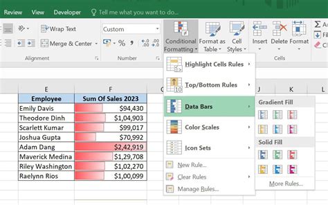
Conditional formatting in Excel is a powerful tool that allows users to highlight cells based on specific conditions, making it easier to analyze and understand data. One common use of conditional formatting is to compare two columns and highlight differences or similarities between them. This can be particularly useful in data analysis, where identifying discrepancies or patterns between different datasets is crucial.

Conditional formatting can help in various scenarios, such as identifying duplicate or unique values, highlighting cells that contain specific text, or formatting cells based on the values in another column. When comparing two columns, the goal is often to visually identify which rows have matching or mismatching values, which can be achieved through a few straightforward steps in Excel.

To get started with comparing two columns using conditional formatting, it's essential to understand the basic principles of how conditional formatting works. Excel allows users to apply formatting to a cell or a range of cells based on a specific condition, such as the cell's value, the value of another cell, or a formula that evaluates to true or false.

When comparing two columns, the most common approach is to use a formula that checks if the values in the two columns are equal or not equal for each row. This can be done using the IF function or direct comparisons within the conditional formatting rules.

The process of setting up conditional formatting to compare two columns involves selecting the range of cells you want to format, opening the conditional formatting dialog, and then specifying the rule based on a formula. For example, if you want to highlight cells in column A that have a different value than the corresponding cell in column B, you would select column A, go to the Home tab in Excel, click on Conditional Formatting, and then choose "New Rule." You would then select "Use a formula to determine which cells to format," and enter a formula like =A1<>B1, assuming you're starting from row 1.

After entering the formula, you click on the "Format" button to choose how you want the cells to be highlighted, such as filling them with a certain color. Finally, you click "OK" to apply the rule. Excel then applies the formatting to the selected range based on the condition specified in the formula.

One of the key benefits of using conditional formatting to compare two columns is its dynamic nature. As the data in the columns changes, the formatting updates automatically, reflecting the new comparisons without the need for manual intervention. This makes it an invaluable tool for ongoing data analysis and monitoring.

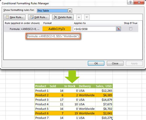
In addition to comparing columns directly, conditional formatting can also be used in more complex scenarios, such as comparing values across multiple columns or using logical operations to combine conditions. For instance, you might want to highlight rows where the value in column A is greater than the value in column B and simultaneously less than the value in column C.

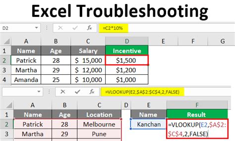
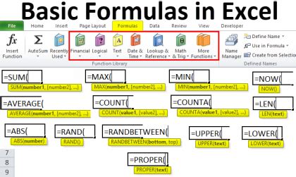
To take full advantage of conditional formatting for comparing two columns, it's helpful to be familiar with Excel's formula capabilities, especially those related to logical and comparison operations. Understanding how to use the IF function, logical operators like AND and OR, and comparison operators like =, <>, >, <, >=, and <= can significantly enhance your ability to create complex and useful conditional formatting rules.

Moreover, conditional formatting is not limited to simple visual changes like background color or font color. You can also use it to apply more complex formatting, such as changing the font style, adding borders, or even using icons to represent different conditions, which can be particularly useful for creating dashboards or reports that need to convey information quickly and intuitively.

Benefits of Using Conditional Formatting

Conditional formatting offers several benefits when comparing two columns or analyzing data in general. It enhances data visualization, making it easier to spot trends, discrepancies, or patterns within the data. This can significantly reduce the time spent on data analysis, as key information is highlighted upfront.

Moreover, conditional formatting is flexible and can be adjusted as needed. Rules can be easily modified, added, or removed, allowing for quick adaptation to changing analysis requirements. This flexibility, combined with its ease of use, makes conditional formatting a preferred method for data analysis among Excel users.

Another significant advantage of conditional formatting is its ability to handle large datasets efficiently. Unlike manual formatting, which can be time-consuming and prone to errors, especially with large datasets, conditional formatting applies rules uniformly across the selected range, ensuring consistency and accuracy.

Common Applications of Conditional Formatting

Conditional formatting has a wide range of applications in data analysis and business intelligence. It can be used to highlight important information, such as deadlines, milestones, or critical thresholds, in project management spreadsheets. In financial analysis, it can help identify trends in revenue, expenses, or profits over time, or highlight cells that exceed budget limits.

In inventory management, conditional formatting can be used to indicate low stock levels, track the status of orders, or identify products that are nearing their expiration dates. This real-time visibility into inventory status can help businesses make informed decisions about restocking, promotions, and product lifecycle management.

Step-by-Step Guide to Conditional Formatting

To apply conditional formatting to compare two columns, follow these steps:

Select the Range: Choose the range of cells you want to format. This could be an entire column, a row, or a specific range of cells.
Open Conditional Formatting: Go to the Home tab in Excel, find the Styles group, and click on Conditional Formatting.
New Rule: Select "New Rule" from the dropdown menu. This opens the New Formatting Rule dialog box.
Use a Formula: Choose "Use a formula to determine which cells to format." This option allows you to specify a custom formula for the rule.
Enter the Formula: In the formula box, enter your comparison formula. For example, to compare values in columns A and B, you might use =A1<>B1.
Format: Click the "Format" button to choose how you want to format the cells that meet the condition. You can select a fill color, font color, and more.
Apply: Click "OK" to apply the rule. Excel will then format the cells in your selected range based on the condition you specified.

Tips for Advanced Conditional Formatting

For more advanced uses of conditional formatting, consider the following tips:

Use Relative References: When entering formulas for conditional formatting, use relative references (like A1) instead of absolute references (like $A$1) so that the formula applies correctly to each cell in the range.
Combine Conditions: You can combine multiple conditions using logical operators like AND, OR, and NOT to create more complex rules.
Apply Multiple Rules: Excel allows you to apply multiple conditional formatting rules to the same range. Rules are applied in the order they appear in the list, so you can adjust the order if necessary.
Use Conditional Formatting with Other Excel Tools: Conditional formatting can be used in conjunction with other Excel tools, such as pivot tables, charts, and filters, to create powerful and dynamic dashboards.

Best Practices for Conditional Formatting

To get the most out of conditional formatting and ensure that your worksheets remain organized and easy to understand, follow these best practices:

Keep it Simple: Avoid overly complex rules that might be hard to understand or maintain. Break down complex conditions into simpler, more manageable parts if necessary.
Use Clear and Consistent Formatting: Apply consistent formatting throughout your worksheet to make it easier to understand at a glance. Use colors and formats that contrast well with your worksheet's background and other elements.
Test Your Rules: Always test your conditional formatting rules with sample data to ensure they work as expected before applying them to your actual data.
Document Your Rules: If you're working on a shared worksheet or one that will be used by others, consider documenting the conditional formatting rules you've applied. This can help others understand the logic behind the formatting and make adjustments as needed.

Common Issues with Conditional Formatting

While conditional formatting is a powerful tool, there are some common issues users may encounter:

Rules Not Applying Correctly: If rules are not applying as expected, check that the formula is correct, the format is properly defined, and the rule is applied to the correct range.
Conflicting Rules: If multiple rules are applied to the same range, they might conflict. Adjust the order of the rules or modify them to ensure they work together as intended.
Performance Issues: Applying too many conditional formatting rules, especially to large datasets, can impact Excel's performance. Limit the number of rules and apply them only where necessary.

Conclusion and Next Steps

Conditional formatting is a versatile and powerful feature in Excel that can significantly enhance data analysis and visualization. By comparing two columns and highlighting differences or similarities, users can quickly identify key trends and patterns within their data. Whether you're a beginner or an advanced Excel user, mastering conditional formatting can take your data analysis skills to the next level.

To further explore the capabilities of conditional formatting and Excel in general, consider diving deeper into advanced formulas, data visualization techniques, and how to integrate Excel with other tools and platforms for more comprehensive data analysis and business intelligence solutions.

Excel Conditional Formatting Image Gallery

What is conditional formatting in Excel?

Conditional formatting is a feature in Excel that allows users to highlight cells based on specific conditions, making it easier to analyze and understand data.

How do I apply conditional formatting to compare two columns?

To apply conditional formatting, select the range of cells, go to the Home tab, click on Conditional Formatting, choose "New Rule," and then select "Use a formula to determine which cells to format." Enter a comparison formula, such as =A1<>B1, and then format the cells as desired.

What are some common applications of conditional formatting?

Conditional formatting has a wide range of applications, including highlighting important information, identifying trends, and tracking the status of projects or inventory. It can be used in financial analysis, project management, and inventory management, among other areas.

We hope this comprehensive guide to using conditional formatting in Excel to compare two columns has been informative and helpful. Whether you're looking to enhance your data analysis skills, create more dynamic and informative spreadsheets, or simply make your data more visually appealing, conditional formatting is a powerful tool that can help you achieve your goals. Feel free to share your thoughts, ask questions, or explore more topics related to Excel and data analysis in the comments below.