Intro
Master Excels Vlookup with multiple criteria using 5 expert methods, including index-match, array formulas, and more, to streamline data analysis and lookup tasks with ease and accuracy.
The Vlookup function is a powerful tool in Excel that allows users to search for a value in a table and return a corresponding value from another column. However, the traditional Vlookup function has limitations, particularly when it comes to searching for multiple criteria. In this article, we will explore five ways to perform a Vlookup with multiple criteria, making it easier to manage complex data sets.
When working with large datasets, it's common to need to search for multiple criteria to find the desired information. This can be challenging with the traditional Vlookup function, which only allows for a single search criterion. Fortunately, there are several ways to overcome this limitation, and we will delve into each of these methods in detail.
The ability to perform a Vlookup with multiple criteria is essential in various fields, including finance, marketing, and operations. By using these techniques, users can streamline their workflow, reduce errors, and make more informed decisions. Whether you're a seasoned Excel user or just starting to explore its capabilities, this article will provide you with the knowledge and skills to take your data analysis to the next level.
Understanding the Vlookup Function
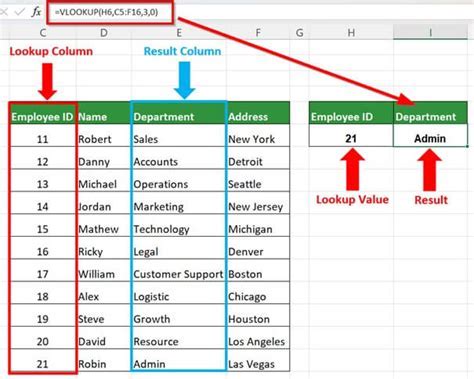
Before we dive into the methods for performing a Vlookup with multiple criteria, it's essential to understand the basics of the Vlookup function. The Vlookup function has four arguments: the value to search for, the table to search in, the column to return a value from, and an optional range lookup argument. The syntax for the Vlookup function is: VLOOKUP(lookup_value, table_array, col_index_num, [range_lookup]).
How the Vlookup Function Works
The Vlookup function works by searching for the lookup value in the first column of the table array. When it finds a match, it returns the corresponding value from the specified column index. If the range lookup argument is set to FALSE, the function will only return an exact match. If it's set to TRUE or omitted, the function will return an approximate match.Method 1: Using the Index-Match Function
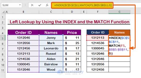
One way to perform a Vlookup with multiple criteria is by using the Index-Match function combination. This method is more flexible and powerful than the traditional Vlookup function. The syntax for the Index-Match function is: INDEX(range, MATCH(lookup_value, lookup_array, [match_type])).
To use the Index-Match function with multiple criteria, you can use the following formula: INDEX(return_range, MATCH(1, (criteria1_range=criteria1) * (criteria2_range=criteria2), 0)). This formula will return the value from the return range that matches both criteria.
Example of Using the Index-Match Function
Suppose you have a table with sales data, and you want to find the sales amount for a specific region and product. You can use the Index-Match function with multiple criteria to achieve this.| Region | Product | Sales |
|---|---|---|
| North | A | 100 |
| North | B | 200 |
| South | A | 50 |
| South | B | 150 |
Using the formula: INDEX(C:C, MATCH(1, (A:A="North") * (B:B="A"), 0)), you can find the sales amount for the North region and product A.
Method 2: Using the Filter Function
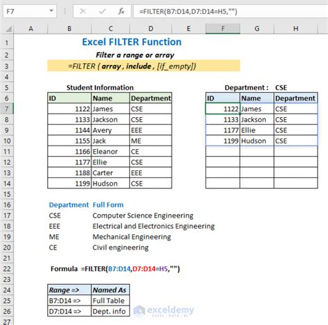
Another way to perform a Vlookup with multiple criteria is by using the Filter function. The Filter function is a new function in Excel that allows you to filter a range of data based on multiple criteria. The syntax for the Filter function is: FILTER(range, criteria_range=criteria).
To use the Filter function with multiple criteria, you can use the following formula: FILTER(return_range, (criteria1_range=criteria1) * (criteria2_range=criteria2)). This formula will return the values from the return range that match both criteria.
Example of Using the Filter Function
Suppose you have a table with customer data, and you want to find the customers who live in a specific city and have a specific job title. You can use the Filter function with multiple criteria to achieve this.| Name | City | Job Title |
|---|---|---|
| John | New York | Manager |
| Jane | Los Angeles | Engineer |
| Bob | New York | Engineer |
| Alice | Los Angeles | Manager |
Using the formula: FILTER(C:C, (B:B="New York") * (D:D="Manager")), you can find the customers who live in New York and have the job title Manager.
Method 3: Using the Vlookup Function with Multiple Criteria Ranges
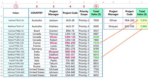
You can also perform a Vlookup with multiple criteria by using the Vlookup function with multiple criteria ranges. This method involves creating a helper column that combines the multiple criteria ranges into a single range.
To use the Vlookup function with multiple criteria ranges, you can use the following formula: VLOOKUP(lookup_value, CHOOSE({1,2}, criteria1_range, criteria2_range), return_col, FALSE). This formula will return the value from the return column that matches both criteria.
Example of Using the Vlookup Function with Multiple Criteria Ranges
Suppose you have a table with order data, and you want to find the order status for a specific customer and order date. You can use the Vlookup function with multiple criteria ranges to achieve this.| Customer | Order Date | Order Status |
|---|---|---|
| John | 2022-01-01 | Pending |
| Jane | 2022-01-02 | Shipped |
| Bob | 2022-01-01 | Pending |
| Alice | 2022-01-02 | Delivered |
Using the formula: VLOOKUP(lookup_value, CHOOSE({1,2}, A:A, B:B), 3, FALSE), you can find the order status for the customer John and order date 2022-01-01.
Method 4: Using the Xlookup Function
The Xlookup function is a new function in Excel that allows you to search for a value in a table and return a corresponding value from another column. The Xlookup function is more flexible and powerful than the traditional Vlookup function.
To use the Xlookup function with multiple criteria, you can use the following formula: XLOOKUP(lookup_value, criteria1_range, return_range, criteria2_range, return_col). This formula will return the value from the return range that matches both criteria.
Example of Using the Xlookup Function
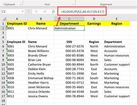
Suppose you have a table with employee data, and you want to find the employee's department for a specific name and job title. You can use the Xlookup function with multiple criteria to achieve this.| Name | Job Title | Department |
|---|---|---|
| John | Manager | Sales |
| Jane | Engineer | IT |
| Bob | Manager | Marketing |
| Alice | Engineer | IT |
Using the formula: XLOOKUP(lookup_value, A:A, C:C, B:B, "Manager"), you can find the department for the employee John and job title Manager.
Method 5: Using Power Query

Power Query is a powerful tool in Excel that allows you to import, transform, and analyze data from various sources. You can use Power Query to perform a Vlookup with multiple criteria by creating a query that filters the data based on the multiple criteria.
To use Power Query with multiple criteria, you can use the following steps:
- Go to the Data tab and click on From Table/Range.
- Select the table that you want to filter.
- Click on the Add Column tab and select the Custom Column option.
- Enter the formula: = Table.Filter(YourTable, each [Criteria1] = "Value1" and [Criteria2] = "Value2").
- Click on the OK button.
Example of Using Power Query
Suppose you have a table with sales data, and you want to find the sales amount for a specific region and product. You can use Power Query to achieve this.| Region | Product | Sales |
|---|---|---|
| North | A | 100 |
| North | B | 200 |
| South | A | 50 |
| South | B | 150 |
Using the formula: = Table.Filter(YourTable, each [Region] = "North" and [Product] = "A"), you can find the sales amount for the North region and product A.
Vlookup Multiple Criteria Image Gallery


What is the Vlookup function in Excel?
+The Vlookup function is a powerful tool in Excel that allows users to search for a value in a table and return a corresponding value from another column.
How do I perform a Vlookup with multiple criteria in Excel?
+There are several ways to perform a Vlookup with multiple criteria in Excel, including using the Index-Match function, the Filter function, the Vlookup function with multiple criteria ranges, the Xlookup function, and Power Query.
What is the syntax for the Index-Match function in Excel?
+The syntax for the Index-Match function is: INDEX(range, MATCH(lookup_value, lookup_array, [match_type])).
In conclusion, performing a Vlookup with multiple criteria in Excel can be achieved through various methods, including using the Index-Match function, the Filter function, the Vlookup function with multiple criteria ranges, the Xlookup function, and Power Query. By understanding these methods and their applications, users can streamline their workflow, reduce errors, and make more informed decisions. We encourage you to try out these methods and explore the capabilities of Excel to improve your data analysis skills. If you have any questions or need further assistance, please don't hesitate to comment or share this article with others.