Excel Format Cell Based On Another Cell

When working with Excel, formatting cells based on the values or contents of another cell can be incredibly useful for highlighting important information, creating visual cues, and making your spreadsheets more intuitive. Excel offers several ways to achieve this, including using Conditional Formatting, formulas, and even VBA scripts for more complex scenarios. Here, we'll explore how to format a cell based on another cell's value using Conditional Formatting, which is one of the most straightforward and powerful methods Excel provides.

Understanding Conditional Formatting

Conditional Formatting is a feature in Excel that allows you to apply formats to a cell or a range of cells based on certain conditions. These conditions can be based on the cell's value, the value of another cell, or even more complex conditions that involve formulas. The feature is accessible through the Home tab on the Excel Ribbon.

Basic Steps to Format a Cell Based on Another Cell

Select the Cell or Range: Click on the cell or select the range of cells you want to format. This is where the formatting will be applied based on the condition you set.
Open Conditional Formatting: Go to the Home tab on the Excel Ribbon, find the Styles group, and click on Conditional Formatting.
New Rule: From the Conditional Formatting dropdown menu, select "New Rule". This opens the New Formatting Rule dialog box.
Use a Formula to Determine Which Cells to Format: In the New Formatting Rule dialog, select "Use a formula to determine which cells to format".
Enter the Formula: In the formula box, you will enter a formula that refers to the cell or cells you want to base your formatting on. For example, if you want to format cell A1 based on the value in cell B1, your formula might look something like =B1>10. This formula will apply the formatting to cell A1 if the value in B1 is greater than 10.
Format: Click on the "Format" button to choose how you want the cell(s) to be formatted when the condition is met. You can choose fill color, font color, number formatting, and more.
Apply: Click OK to apply your rule. The formatting will now be applied to the selected cell(s) based on the condition you specified.

Examples of Conditional Formatting Formulas

Format Cell A1 if Cell B1 is Greater Than 10: =B1>10
Format Cell A1 if Cell B1 Contains the Text "Yes": =ISNUMBER(SEARCH("Yes",B1))
Format Cell A1 if Cell B1 is Less Than or Equal to 5: =B1<=5
Format Cell A1 if Cell B1 is Blank: =ISBLANK(B1)
Format Cell A1 if Cell B1 is Not Blank: =NOT(ISBLANK(B1))

Using Multiple Conditions

If you need to apply formatting based on multiple conditions, you can use the "AND" and "OR" functions within your formula. For example:

Format Cell A1 if Cell B1 is Greater Than 10 and Cell C1 is Less Than 5: =AND(B1>10, C1<5)
Format Cell A1 if Cell B1 is Greater Than 10 or Cell C1 is Less Than 5: =OR(B1>10, C1<5)

Tips and Variations

Applying to Entire Rows or Columns: You can apply Conditional Formatting to entire rows or columns based on the values in specific cells within those rows or columns. Simply adjust your formula to reference the appropriate cells.
Using Relative and Absolute References: Be mindful of whether you're using relative or absolute references in your formulas. Absolute references (denoted by $ signs, e.g., $B$1) are useful when you want to format a range of cells based on a single cell's value.
Managing Rules: If you apply multiple rules, you can manage them through the Conditional Formatting menu by selecting "Manage Rules". This allows you to edit, delete, or reorder your rules.

Advanced Conditional Formatting Techniques

For more complex formatting needs, consider exploring Excel's other features, such as:

IF Functions: Useful for creating more complex conditions that involve multiple outcomes.
VBA Macros: Allow for highly customized and automated formatting tasks, especially useful for large datasets or repetitive tasks.
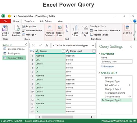
Power Query: Can be used to transform and format data in powerful ways, especially when dealing with large datasets.

Gallery of Excel Formatting Techniques

Excel Formatting Techniques Image Gallery

FAQs

What is Conditional Formatting in Excel?

Conditional Formatting is a feature that allows you to apply formats to a cell or range of cells based on specific conditions.

How Do I Apply Conditional Formatting Based on Another Cell?

Select the cell or range to format, go to Home > Conditional Formatting, select New Rule, and then use a formula to determine which cells to format.

Can I Use Multiple Conditions for Conditional Formatting?

Yes, you can use the AND and OR functions within your formula to apply formatting based on multiple conditions.

In conclusion, formatting cells based on another cell's value in Excel is a powerful feature that can significantly enhance the usability and visual appeal of your spreadsheets. By mastering Conditional Formatting and exploring more advanced techniques, you can create dynamic, interactive spreadsheets that communicate complex information more effectively. Whether you're a beginner or an advanced user, leveraging these capabilities can take your Excel skills to the next level and make you more efficient in your work. So, dive in, experiment with different formulas and conditions, and see how Conditional Formatting can transform your spreadsheet experience.