Excel List All Values That Match Criteria

When working with large datasets in Excel, it's often necessary to filter and identify specific values that match certain criteria. Excel provides several methods to achieve this, including using formulas, filters, and pivot tables. Here, we'll explore how to list all values that match specific criteria using these methods.

The ability to list values based on criteria is crucial for data analysis, reporting, and decision-making. Whether you're working with sales data, customer information, or inventory levels, being able to quickly and accurately identify relevant data points is essential.

Introduction to Excel's Filtering Capabilities

Excel offers powerful filtering capabilities that allow users to narrow down their data to show only the rows that meet specific conditions. This can be done through the use of filters, which can be applied to one or more columns to display only the data that matches the specified criteria.

Using AutoFilter

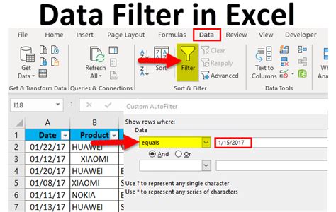
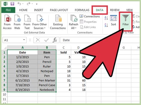
1. Select Your Data: Begin by selecting the entire range of cells that contains the data you want to filter, including headers.
2. Apply AutoFilter: Go to the "Data" tab on the Ribbon and click on the "Filter" button. This will add filter arrows to the headers of your selected range.
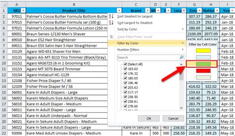
3. Filter Your Data: Click on the filter arrow in the column you want to apply the filter to, and then select "Text Filters" or "Number Filters" depending on the type of data in that column. Choose the specific filter option that matches your criteria (e.g., "Equals", "Does Not Equal", "Greater Than", etc.).
4. Apply the Filter: After selecting your filter criteria, click "OK". Excel will then display only the rows that match your specified condition.

Using Formulas to List Values

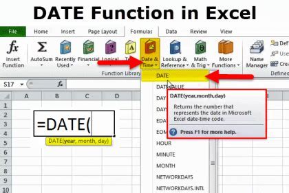
If you need a more dynamic or flexible way to list values that match certain criteria, using formulas can be an effective approach. Excel's IF function, combined with filtering, or more advanced functions like FILTER (available in Excel 2019 and later versions), can help achieve this.

Using the IF Function

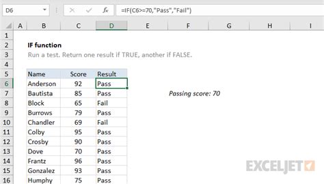
The IF function can be used to test a condition and return one value if true and another value if false. While it doesn't directly list values, it can be used in conjunction with filtering to highlight or separate data based on criteria.

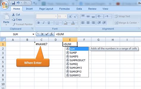
1. Enter the IF Formula: In a new column, enter a formula like =IF(A2>10, "Greater than 10", "Less than or equal to 10"), assuming your data is in column A and you're checking if the value in cell A2 is greater than 10.
2. Copy the Formula Down: Drag the fill handle (small square at the bottom-right corner of the cell) down to apply the formula to all relevant cells.
3. Filter the Results: Use the AutoFilter feature on this new column to show only the rows that match your desired condition.

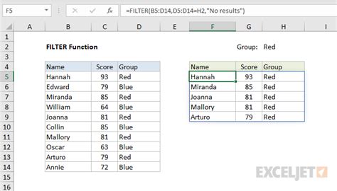
Using the FILTER Function

The FILTER function is a more direct way to return values that meet specific criteria. It's available in Excel 2019 and later versions.

1. Enter the FILTER Formula: Suppose you want to list all values in column A that are greater than 10. You could use a formula like =FILTER(A:A, A:A > 10).
2. Press Enter: Excel will return an array of values from column A that are greater than 10.

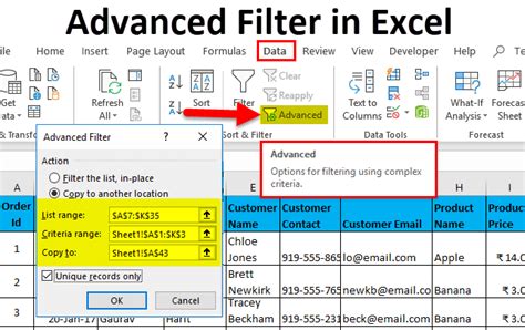
Using PivotTables

PivotTables are another powerful tool in Excel for summarizing and analyzing large datasets. They can also be used to list values that match specific criteria.

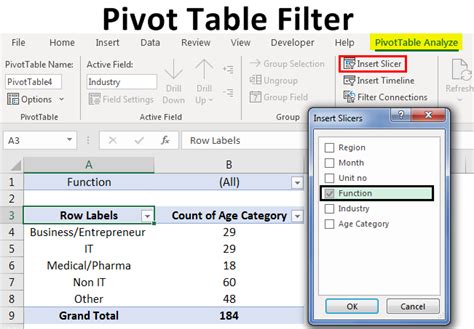
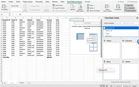
1. Create a PivotTable: Select your data range, go to the "Insert" tab, and click on "PivotTable". Choose a cell to place the PivotTable and click "OK".
2. Drag Fields to Filters: In the PivotTable Fields pane, drag the field you want to filter on to the "Filters" area.
3. Apply Filter: Right-click on the filter field in the PivotTable and select "Filter" > "Select Multiple Items", then choose the items you want to include.

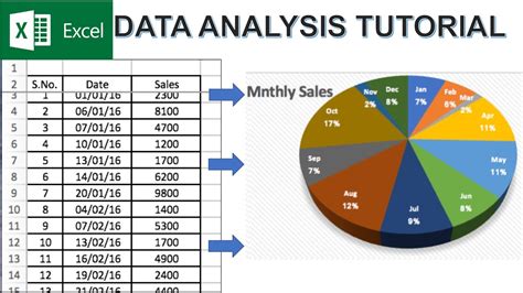
Practical Examples and Statistical Data

• Example 1: Suppose you have a list of sales figures for different products, and you want to identify all products with sales greater than $1,000. Using the FILTER function, you could use =FILTER(B:B, B:B > 1000), assuming sales figures are in column B.
• Example 2: If you're analyzing customer data and want to list all customers from a specific region, you could use AutoFilter on the region column to select the desired region.

Gallery of Excel Filtering Techniques

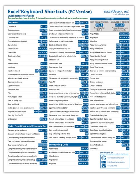
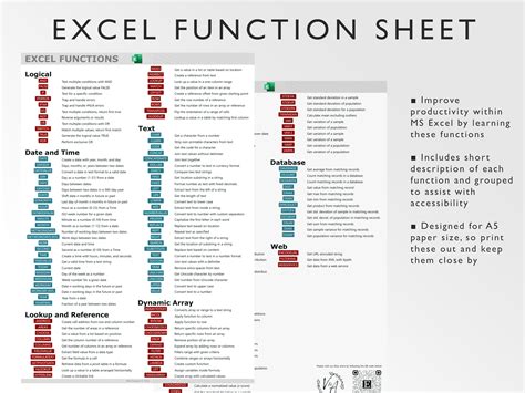
Gallery of Excel Functions

Excel Functions Gallery

FAQs

How do I filter data in Excel to show only specific values?

+

To filter data in Excel, select your data range, go to the "Data" tab, and click on "Filter". Then, use the filter arrows in the headers to select the criteria you want to apply.

What is the difference between the IF and FILTER functions in Excel?

+

The IF function tests a condition and returns one value if true and another if false. The FILTER function returns an array of all values that meet the specified condition.

How do I use PivotTables to list values that match specific criteria?

+

Create a PivotTable from your data, drag the field you want to filter on to the "Filters" area, and then apply the filter as needed.

In conclusion, listing all values that match specific criteria in Excel can be efficiently achieved through various methods, including AutoFilter, the use of formulas like IF and FILTER, and the application of PivotTables. Each method has its advantages and can be chosen based on the complexity of the data and the specific requirements of the analysis. By mastering these techniques, users can enhance their data analysis capabilities and make more informed decisions. We invite you to share your experiences with filtering data in Excel and any tips you might have for our readers.