Intro
The ability to convert month names to numbers in Excel is a valuable skill, especially when working with datasets that include dates or months in text format. This conversion can be crucial for various data analysis tasks, such as sorting, filtering, or performing calculations based on the month. Excel offers several methods to achieve this conversion, catering to different scenarios and user preferences. Here, we'll explore five ways to convert month names to numbers in Excel, highlighting their application, benefits, and step-by-step instructions.
To begin with, understanding why converting month names to numbers is important can help in appreciating the methods discussed. Month names are often used in reports, charts, and tables for better readability, but when it comes to calculations or arranging data in chronological order, numerical representations are more practical. Excel, being a powerful tool for data management and analysis, provides multiple functions and techniques to facilitate this conversion.
Introduction to Excel Functions
Before diving into the methods, it's essential to familiarize yourself with Excel functions and formulas. Excel functions are predefined formulas that perform specific calculations, such as converting text to numbers, which is the focus of our discussion. These functions can be combined and nested to achieve complex data transformations and analyses.
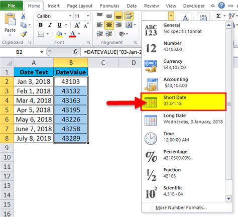
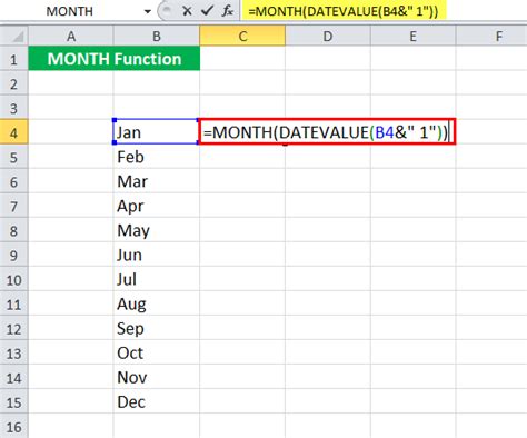
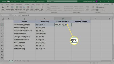
Method 1: Using the MONTH and DATEVALUE Functions
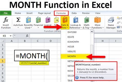
- Assume the month name is in cell A1.
- Use the formula
=MONTH(DATEVALUE(A1&" 1"))to convert the month name to a number. - The
&" 1"part adds " 1" to the month name to create a date string that Excel can recognize (e.g., "January 1").
Method 2: Using VLOOKUP
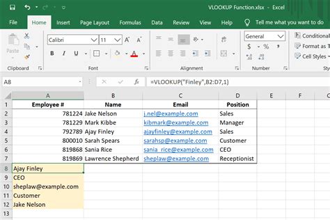
- Create a table with month names in one column and their corresponding numbers in the next column.
- Use the VLOOKUP formula, such as
=VLOOKUP(A1, B:C, 2, FALSE), where A1 is the cell with the month name, B:C is the range of the table, and 2 specifies that the function should return the value in the second column.
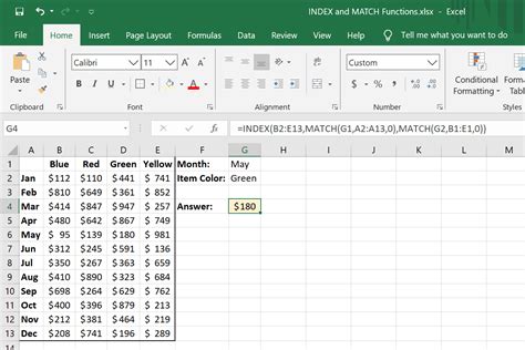
Method 3: Using INDEX and MATCH Functions
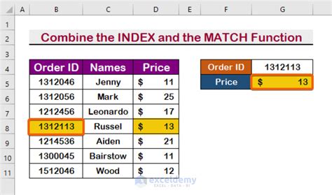
- Similar to the VLOOKUP method, create a table with month names and numbers.
- Use the formula
=INDEX(C:C, MATCH(A1, B:B, 0)), where A1 is the cell with the month name, B:B is the column with the month names, and C:C is the column with the month numbers.
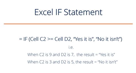
Method 4: Using IF Functions

- Start with
=IF(A1="January", 1, IF(A1="February", 2,...))and continue for all 12 months. - This method is less efficient for large datasets due to its complexity and the character limit in Excel formulas.
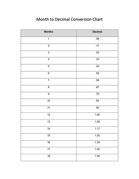
Method 5: Using CHOOSE and MATCH Functions

- Use the formula
=CHOOSE(MATCH(A1, {"January", "February", "March", "April", "May", "June", "July", "August", "September", "October", "November", "December"}, 0), 1, 2, 3, 4, 5, 6, 7, 8, 9, 10, 11, 12). - This formula matches the month name in A1 with the list of months and returns the corresponding number based on the position in the list.
Gallery of Excel Functions for Month Conversion
Excel Functions Gallery


Frequently Asked Questions
What is the most efficient way to convert month names to numbers in Excel?
+The most efficient method depends on the specific scenario. For most cases, using the MONTH and DATEVALUE functions or the VLOOKUP function is recommended due to their simplicity and flexibility.
Can I use these methods for converting month names in other languages?
+Yes, but you might need to adjust the formulas to accommodate the language differences, especially when using text-based functions like VLOOKUP or INDEX/MATCH.
How do I handle errors or #N/A values when converting month names to numbers?
+You can use error-handling functions like IFERROR or IFNA to manage errors and return a custom value or message instead of the error.
In conclusion, converting month names to numbers in Excel is a straightforward process once you're familiar with the available functions and methods. Each method has its advantages and can be chosen based on the specific requirements of your project or personal preference. By mastering these techniques, you can efficiently manage and analyze date-related data in Excel, making your workflow more productive and your data insights more meaningful. Feel free to share your experiences or ask further questions about working with dates in Excel in the comments below.