Excel Sumif Filtered Rows Formula

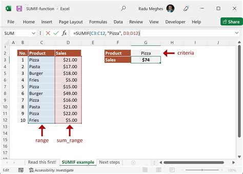
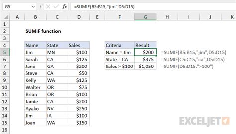
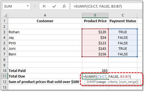
The Excel Sumif function is a powerful tool used to sum values in a specific range of cells, based on criteria that you specify. However, when dealing with filtered rows, the traditional Sumif function may not work as expected because it sums values from all rows, regardless of whether they are filtered or not. To sum values from only the visible or filtered rows, you can use a combination of functions, including the Sumproduct and Subtotal functions. In this article, we will delve into the details of how to create an Excel Sumif formula for filtered rows, exploring the different methods and providing examples to help you understand the process better.

When working with large datasets in Excel, filtering data is a common practice to focus on specific subsets of information. However, performing calculations on filtered data can be challenging because Excel's standard functions often ignore the filter and include all data in their calculations. To overcome this, you need to use functions that are sensitive to the filter status of rows. Let's explore how to sum values in filtered rows using different approaches.

Understanding the Challenge

The primary challenge with summing filtered rows is that Excel's built-in Sumif function does not differentiate between visible and hidden rows when a filter is applied. This means that even if you filter your data to show only certain rows, the Sumif function will still include values from all rows in its calculation, not just the ones that are visible.

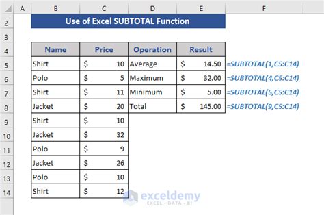
Solution 1: Using the Subtotal Function

One of the simplest ways to sum only the visible rows after applying a filter is by using the Subtotal function. The Subtotal function is specifically designed to work with filtered data, making it an ideal choice for this task.

To use the Subtotal function, follow these steps:

Select the cell where you want to display the sum.
Type =SUBTOTAL(109, followed by the range of cells you want to sum.
Close the parenthesis and press Enter.

The number 109 in the Subtotal function tells Excel to sum the values in the specified range, ignoring any hidden rows due to filtering.

Solution 2: Using the Sumproduct Function

Another approach to summing filtered rows involves using the Sumproduct function in combination with the Filterxml function (in Excel 2019 and later versions) or by leveraging the properties of the Sumproduct function itself to ignore hidden rows.

For Excel versions prior to 2019, you can use the Sumproduct function in a creative way to sum visible cells only. However, this method is more complex and typically involves using helper columns or arrays, which can be cumbersome for large datasets.

Solution 3: Using the Filter Function (Excel 365 and Later)

In Excel 365 and later versions, the Filter function provides a straightforward way to sum values based on conditions, including the visibility of rows. However, this function is part of the dynamic array formulas, which are only available in the latest versions of Excel.

To sum filtered rows using the Filter function, you would typically use a formula that looks something like this:

=SUM(FILTER(range, condition))

Where range is the range of cells you want to sum, and condition specifies the criteria for which rows to include in the sum.

Practical Examples

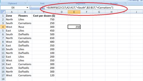
Let's consider a practical example to illustrate how these solutions work. Suppose you have a list of sales data with columns for the region, product, and sales amount, and you want to sum the sales amounts for a specific region after filtering the data.

Example 1: Using Subtotal

Assuming your sales data is in the range A1:C100, and you've filtered the data to show only rows for the "North" region, you can use the Subtotal function like this:

=SUBTOTAL(109, C2:C100)

This formula sums the sales amounts in column C, ignoring any hidden rows due to the filter.

Example 2: Using Sumproduct

For a more complex scenario or in earlier versions of Excel where the Subtotal function might not be suitable, you might consider using the Sumproduct function. However, this approach often requires additional steps or helper columns, making it less straightforward than using the Subtotal function.

Example 3: Using Filter (Excel 365 and Later)

If you're using Excel 365 or a later version, you can leverage the Filter function to sum values based on specific conditions, including the visibility of rows. This approach provides a flexible and powerful way to work with filtered data.

Benefits of Using Sumif for Filtered Rows

Using the Sumif function or its alternatives for summing filtered rows offers several benefits, including:

Accuracy: By only summing visible rows, you ensure that your calculations reflect the current state of your filtered data.
Flexibility: These functions allow you to work dynamically with your data, adapting to changes in your filter criteria.
Efficiency: Once set up, these formulas save time by automatically updating when your filter changes.

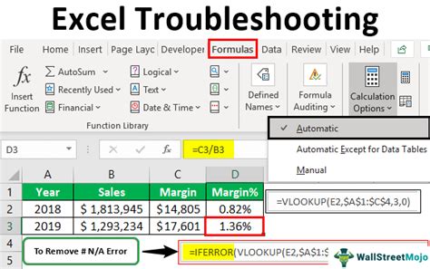
Common Errors and Troubleshooting

When working with formulas to sum filtered rows, you might encounter a few common issues:

#VALUE! Errors: These can occur if your formula references a range that includes non-numeric data. Ensure that your range only includes numbers.
Incorrect Results: Double-check that your filter is applied correctly and that your formula is referencing the correct range.

Step-by-Step Guide to Implementing Sumif for Filtered Rows

Prepare Your Data: Ensure your data is organized in a table format with clear headers.
Apply a Filter: Use Excel's filter feature to narrow down your data based on your criteria.
Choose a Method: Decide which method (Subtotal, Sumproduct, or Filter) best suits your needs based on your Excel version and data complexity.
Write Your Formula: Carefully construct your formula, ensuring you reference the correct range and apply the appropriate criteria.
Test Your Formula: Verify that your formula returns the expected results by checking it against manual calculations or expected outcomes.

Advanced Techniques for Summing Filtered Rows

For more complex scenarios, you might need to combine multiple functions or use array formulas to achieve your desired outcome. Advanced techniques can include:

Using Helper Columns: Creating additional columns to help apply complex criteria to your sum.
Array Formulas: Utilizing array formulas to perform calculations on arrays of data, which can be particularly useful when dealing with filtered data.

Gallery of Excel Sumif Examples

Excel Sumif Image Gallery

Frequently Asked Questions

What is the Sumif function in Excel?

The Sumif function in Excel is used to sum values in a specific range of cells, based on criteria that you specify.

How do I sum only visible cells in Excel?

To sum only visible cells in Excel, you can use the Subtotal function with the argument 109, which tells Excel to sum only the visible cells in the specified range.

What is the difference between Sumif and Subtotal in Excel?

The Sumif function sums values based on criteria, regardless of whether the rows are filtered or not. The Subtotal function, on the other hand, sums values only from the visible rows after applying a filter.

As you've seen, summing filtered rows in Excel can be achieved through various methods, each with its own advantages and suitable scenarios. By mastering these techniques, you can efficiently work with large datasets and perform calculations that reflect the current state of your filtered data. Whether you're using the Subtotal function, Sumproduct, or more advanced techniques, the key to success lies in understanding your data and choosing the right tool for the job. We invite you to share your experiences, ask questions, or provide tips on how you handle summing filtered rows in Excel. Your input can help others and contribute to a more comprehensive understanding of Excel's capabilities.