Excel Vlookup Compare Two Columns

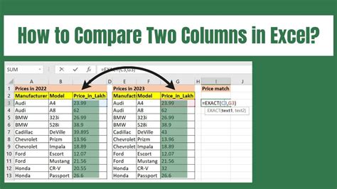
When working with Excel, comparing two columns is a common task, especially when dealing with large datasets. One of the most effective ways to compare two columns in Excel is by using the VLOOKUP function. The VLOOKUP function is designed to look up a value in a table and return a corresponding value from another column. However, it can also be used to compare two columns by looking up values in one column and checking if they exist in another column.

The importance of comparing two columns cannot be overstated, as it allows users to identify matches, duplicates, or unique values between two datasets. This can be crucial in various scenarios, such as data analysis, data cleaning, and data merging. By using the VLOOKUP function to compare two columns, users can streamline their workflow, reduce errors, and make more informed decisions.

In addition to its practical applications, comparing two columns using VLOOKUP also highlights the versatility and power of Excel. With its intuitive interface and extensive range of functions, Excel provides users with a comprehensive toolkit for data management and analysis. By mastering the VLOOKUP function and other Excel tools, users can unlock new possibilities for data analysis and presentation, making it an essential skill for anyone working with data.

Understanding the VLOOKUP Function

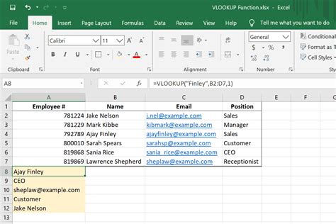
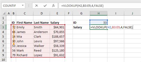
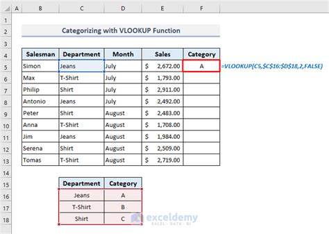
The VLOOKUP function is a powerful tool in Excel that allows users to look up a value in a table and return a corresponding value from another column. The syntax for the VLOOKUP function is: VLOOKUP(lookup_value, table_array, col_index_num, [range_lookup]). The lookup_value is the value that you want to look up, the table_array is the range of cells that contains the data, the col_index_num is the column number that contains the value you want to return, and the [range_lookup] is an optional argument that specifies whether you want an exact match or an approximate match.

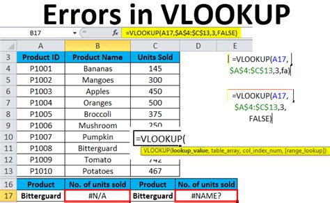
To use the VLOOKUP function to compare two columns, you can look up values in one column and check if they exist in another column. For example, if you have two columns of data, A and B, and you want to check if the values in column A exist in column B, you can use the VLOOKUP function to look up each value in column A and return a corresponding value from column B. If the value is found, the VLOOKUP function will return the value; if not, it will return a #N/A error.

Comparing Two Columns Using VLOOKUP

To compare two columns using VLOOKUP, follow these steps:

Select the cell where you want to display the result.
Type =VLOOKUP( and select the cell that contains the value you want to look up.
Select the range of cells that contains the data you want to search.
Enter the column number that contains the value you want to return.
Close the parenthesis and press Enter.

For example, if you want to compare the values in column A with the values in column B, you can use the following formula: =VLOOKUP(A2, B:B, 1, FALSE). This formula looks up the value in cell A2 and returns the corresponding value from column B. If the value is not found, it returns a #N/A error.

Handling #N/A Errors

When using the VLOOKUP function to compare two columns, you may encounter #N/A errors if the value is not found. To handle these errors, you can use the IFERROR function, which returns a custom value if the formula returns an error. For example, you can use the following formula: =IFERROR(VLOOKUP(A2, B:B, 1, FALSE), "Not found"). This formula returns the value "Not found" if the VLOOKUP function returns a #N/A error.

Alternatively, you can use the IF function to check if the value is found and return a custom value if not. For example, you can use the following formula: =IF(ISERROR(VLOOKUP(A2, B:B, 1, FALSE)), "Not found", VLOOKUP(A2, B:B, 1, FALSE)). This formula checks if the VLOOKUP function returns an error and returns the value "Not found" if true.

Best Practices for Comparing Two Columns

When comparing two columns using VLOOKUP, it's essential to follow best practices to ensure accurate results. Here are some tips:

Make sure the data is clean and free of errors.
Use the correct syntax for the VLOOKUP function.
Use the IFERROR or IF function to handle #N/A errors.
Use the FALSE argument to specify an exact match.
Avoid using the VLOOKUP function with large datasets, as it can slow down your worksheet.

By following these best practices, you can ensure accurate results when comparing two columns using VLOOKUP.

Common Mistakes to Avoid

When using the VLOOKUP function to compare two columns, there are common mistakes to avoid. Here are some of the most common mistakes:

Using the wrong syntax for the VLOOKUP function.
Not specifying the correct column number.
Not using the FALSE argument to specify an exact match.
Not handling #N/A errors.
Using the VLOOKUP function with large datasets.

By avoiding these common mistakes, you can ensure accurate results when comparing two columns using VLOOKUP.

Alternatives to VLOOKUP

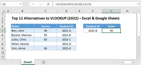
While the VLOOKUP function is a powerful tool for comparing two columns, there are alternatives that can be used in certain situations. Here are some alternatives to VLOOKUP:

INDEX/MATCH function: This function is similar to VLOOKUP but is more flexible and powerful.
LOOKUP function: This function is similar to VLOOKUP but is used for looking up values in a table.
FILTER function: This function is used for filtering data based on certain criteria.

By using these alternatives, you can compare two columns in different ways and achieve more accurate results.

Excel VLOOKUP Image Gallery

What is the VLOOKUP function in Excel?

The VLOOKUP function is a powerful tool in Excel that allows users to look up a value in a table and return a corresponding value from another column.

How do I use the VLOOKUP function to compare two columns?

To use the VLOOKUP function to compare two columns, you can look up values in one column and check if they exist in another column. Use the syntax =VLOOKUP(lookup_value, table_array, col_index_num, [range_lookup]) and specify the correct column number and range lookup.

What are some common mistakes to avoid when using the VLOOKUP function?

Common mistakes to avoid when using the VLOOKUP function include using the wrong syntax, not specifying the correct column number, not using the FALSE argument to specify an exact match, and not handling #N/A errors.

What are some alternatives to the VLOOKUP function?

Alternatives to the VLOOKUP function include the INDEX/MATCH function, the LOOKUP function, and the FILTER function. These functions can be used in certain situations to compare two columns and achieve more accurate results.

How do I handle #N/A errors when using the VLOOKUP function?

To handle #N/A errors when using the VLOOKUP function, you can use the IFERROR function or the IF function to return a custom value if the formula returns an error.

In conclusion, comparing two columns using VLOOKUP is a powerful tool in Excel that can help users identify matches, duplicates, or unique values between two datasets. By following best practices and avoiding common mistakes, users can ensure accurate results and achieve more efficient data analysis. Whether you're a beginner or an advanced user, mastering the VLOOKUP function can unlock new possibilities for data management and analysis. So why not give it a try and see the difference it can make in your workflow? Share your experiences and tips for using VLOOKUP in the comments below, and don't forget to share this article with your colleagues and friends who may benefit from this powerful tool.