Intro
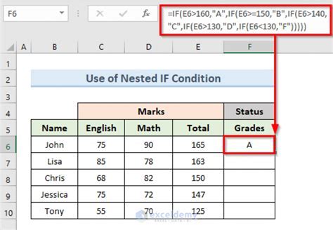
The Vlookup function in Excel is a powerful tool used for looking up and retrieving data from a table or range by matching a value in the first column of the range. However, there are instances where you might need to perform a lookup with multiple conditions, similar to a SQL "WHERE" clause. Excel's Vlookup function alone does not support multiple conditions directly, but you can achieve this by combining Vlookup with other functions or by using alternative methods such as Index/Match, Filter, or even Power Query for more complex scenarios.
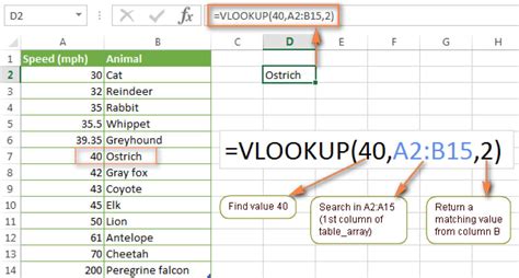
Excel Vlookup's basic syntax is VLOOKUP(lookup_value, table_array, col_index_num, [range_lookup]), where you specify the value to look up, the range of cells to search, the column number that contains the value you want to return, and optionally whether you want an exact or approximate match. But when you need to apply conditions similar to a "WHERE" clause, you have to think beyond the basic Vlookup.
Using Index/Match for Multiple Conditions
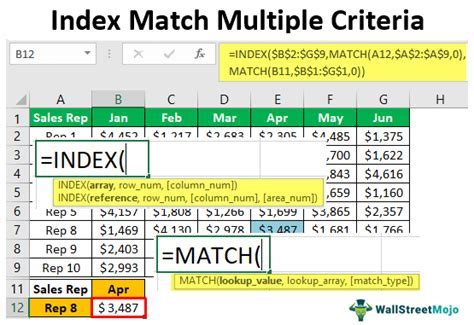
One of the most common and flexible methods to perform lookups with multiple conditions is by using the combination of Index and Match functions. The syntax for this method is INDEX(range1, MATCH(1, (condition1) * (condition2) *..., 0)), where range1 is the range from which you want to return a value, and condition1, condition2, etc., are the conditions you want to apply.
For example, suppose you have a table with names, ages, and cities, and you want to find the age of a person named "John" who lives in "New York". Your table might look like this:
| Name | Age | City |
|---|---|---|
| John | 25 | New York |
| Jane | 30 | Los Angeles |
| John | 28 | Chicago |
You can use the following formula: =INDEX(C:C, MATCH(1, (A:A="John") * (B:B="New York"), 0)), assuming your data is in columns A (Name), B (Age), and C (City). However, this formula has a flaw because it references entire columns, which can lead to errors and slow down your spreadsheet. It's better to define specific ranges, like =INDEX(C2:C100, MATCH(1, (A2:A100="John") * (B2:B100="New York"), 0)).
Using Filter for Multiple Conditions (Excel 365 and Later)
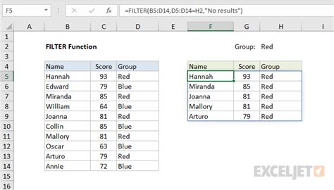
For users with Excel 365 or later versions, the Filter function provides a straightforward way to apply multiple conditions. The syntax for the Filter function is FILTER(range, condition1, [condition2],...), where range is the range of cells that you want to filter, and condition1, condition2, etc., are the conditions you want to apply.
Continuing with the previous example, if you want to find the age of all individuals named "John" who live in "New York", you can use: =FILTER(B:B, (A:A="John") * (C:C="New York")). Again, it's advisable to use specific ranges instead of entire columns for better performance.
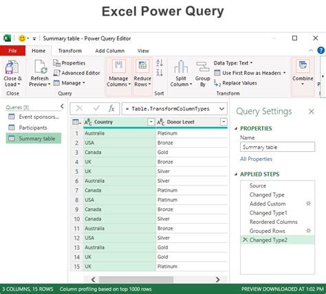
Using Power Query for Complex Lookups
For more complex data analysis and lookups, Power Query (available in Excel 2010 and later versions) offers powerful features. You can load your data into Power Query, apply filters (which act like "WHERE" conditions), and then load the filtered data back into Excel.
- Select your data range and go to the "Data" tab.
- Click "From Table/Range" to load your data into Power Query.
- In the Power Query Editor, you can add filters by clicking on the filter icons in the column headers or by using the "Add Column" tab to create custom filters.
- Once you've applied your filters, click "Close & Load" to load the filtered data into a new worksheet.
Practical Examples and Statistical Data
Let's consider a practical example where we have sales data for different regions, and we want to find the total sales for a specific region and product category.
| Region | Product Category | Sales |
|---|---|---|
| North | Electronics | 1000 |
| South | Electronics | 800 |
| North | Clothing | 1200 |
| South | Clothing | 900 |
To find the total sales of Electronics in the North region, you can use the Index/Match method: =SUMIFS(C:C, A:A, "North", B:B, "Electronics"), assuming your data is in columns A (Region), B (Product Category), and C (Sales).
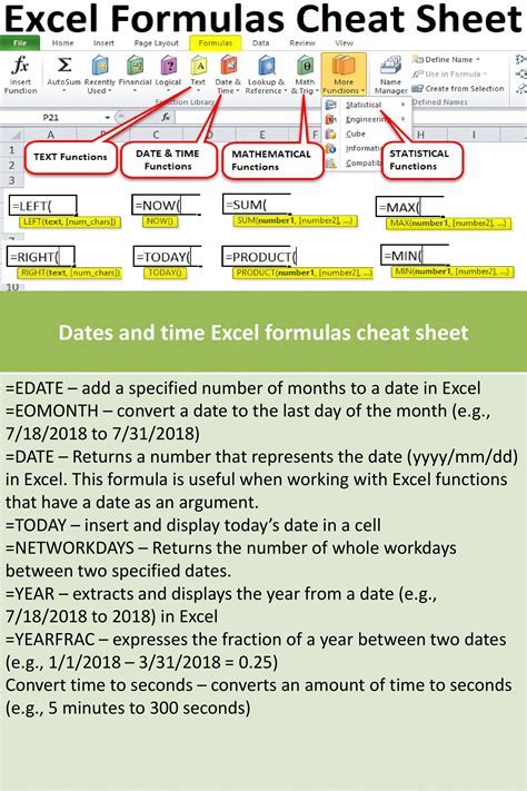
Embedding Images for Better Understanding
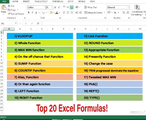
Gallery of Excel Functions
Excel Functions Gallery
FAQs
What is the main difference between Vlookup and Index/Match?
+Vlookup looks up a value in the first column of a table and returns a value in the same row from another column, while Index/Match offers more flexibility by allowing lookups in any column and handling multiple conditions more easily.
How do I apply multiple conditions in the Filter function?
+You can apply multiple conditions by separating them with the asterisk (*) symbol, which acts as a logical AND operator, or by using the Filter function multiple times, each time applying a different condition.
What are the advantages of using Power Query for data analysis?
+Power Query offers powerful data manipulation and analysis capabilities, including the ability to connect to various data sources, apply complex filters, perform data transformations, and load data into Excel for further analysis.
In conclusion, while Excel's Vlookup function is incredibly useful, it has its limitations, especially when dealing with multiple conditions. By leveraging alternative methods such as Index/Match, the Filter function, or Power Query, you can overcome these limitations and perform more complex data lookups and analyses. Whether you're working with simple datasets or complex data models, understanding and mastering these techniques can significantly enhance your productivity and insights in Excel. Feel free to share your experiences or ask further questions in the comments below, and don't forget to share this article with anyone who might benefit from learning more about Excel's powerful lookup and data analysis capabilities.