Google Sheets Conditional Formatting Based On Another Column

Conditional formatting in Google Sheets is a powerful tool that allows you to highlight cells based on specific conditions, making it easier to visualize and analyze your data. One common use case is to apply conditional formatting based on the values in another column. This feature enables you to dynamically change the formatting of cells in one column based on the content of cells in a different column, enhancing the readability and interpretability of your spreadsheet.

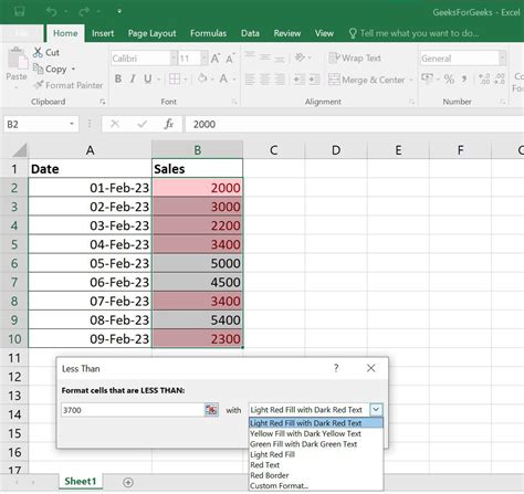
The importance of conditional formatting cannot be overstated, especially in data analysis and reporting. It helps in quickly identifying trends, patterns, and outliers within your dataset. For instance, in a sales report, you might want to highlight cells in a "Sales" column that are above a certain threshold, or in a "Status" column, you might want to color-code different states such as "Pending," "Approved," or "Rejected." By applying conditional formatting based on another column, you can automate this process, ensuring that your spreadsheet updates dynamically as your data changes.

To get started with conditional formatting based on another column in Google Sheets, you first need to understand the basic steps involved. The process typically begins with selecting the range of cells you want to format, then using the conditional formatting tool to set up your rules. Google Sheets provides a straightforward interface for creating these rules, allowing you to specify conditions based on the values in other columns, including the use of formulas for more complex logic.

Setting Up Conditional Formatting

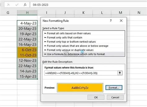
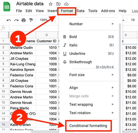
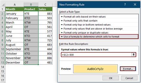
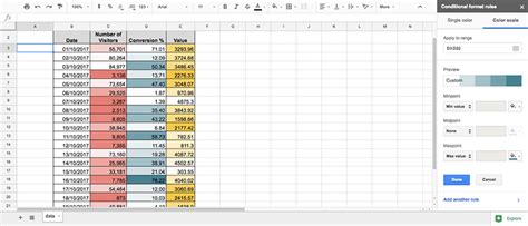
The first step in setting up conditional formatting based on another column is to select the cell or range of cells you want to apply the formatting to. Then, go to the "Format" tab in the menu, and select "Conditional formatting." This will open a sidebar where you can define your formatting rules. In the "Format cells if" dropdown, you can choose from a variety of conditions, including "Custom formula is," which is particularly useful for basing your formatting on values in another column.

Using Custom Formulas

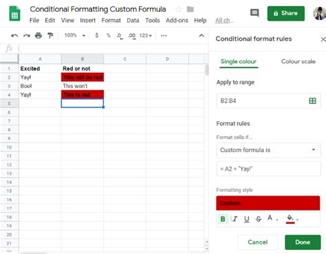
When using custom formulas for conditional formatting, you have the flexibility to reference cells in other columns. For example, if you want to highlight cells in column A based on whether the corresponding cell in column B is greater than a certain value, you can use a formula like =B1>10. This formula checks if the value in cell B1 is greater than 10, and if so, applies the specified formatting to cell A1. You can adjust this formula to fit your specific needs, including referencing entire columns or using more complex logical operations.

Applying Conditional Formatting Based on Another Column

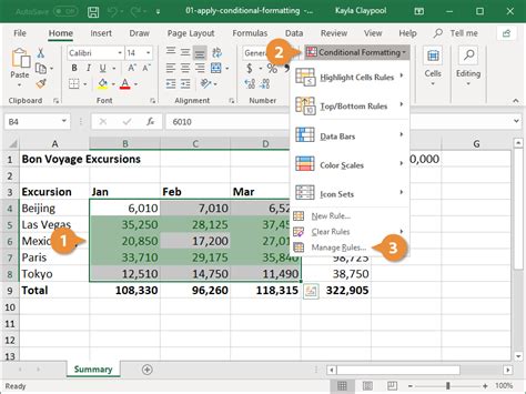
To apply conditional formatting based on another column, follow these steps:

1. Select the range of cells you want to format.
2. Go to the "Format" tab and select "Conditional formatting."
3. In the format cells if dropdown, select "Custom formula is."
4. Enter your custom formula, referencing the other column as needed.
5. Choose your desired formatting options.
6. Click "Done" to apply the rule.

Benefits and Examples

The benefits of using conditional formatting based on another column are numerous. It can help in:

• Data Visualization: By highlighting important trends or values, you can more easily understand your data.
• Error Detection: Conditional formatting can be used to identify errors or inconsistencies in your data.
• Automation: It automates the process of updating cell formats as your data changes, saving time and reducing the chance of human error.

Examples of conditional formatting based on another column include:

• Highlighting sales figures that exceed a certain threshold based on the region.
• Color-coding project statuses based on their current phase.
• Identifying overdue tasks based on their due dates.

Common Formulas and Techniques

Some common formulas and techniques used in conditional formatting based on another column include:

• Comparisons: Using >, <, =, etc., to compare values.
• Logical Operations: Using AND, OR, NOT to combine conditions.
• Referencing Other Columns: Using the column letter in your formula to reference values in other columns.

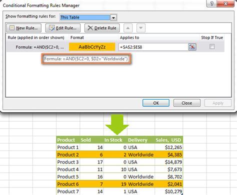
For instance, to highlight cells in column A if the corresponding cell in column B is "Approved," you could use the formula =B1="Approved".

Tips and Best Practices

When working with conditional formatting based on another column, keep the following tips and best practices in mind:

• Keep it Simple: Start with simple conditions and gradually move to more complex ones.
• Test Your Formulas: Always test your custom formulas in a separate cell before applying them to conditional formatting.
• Use Relative References: Unless you specifically need to reference a fixed cell, use relative references (e.g., B1) instead of absolute references (e.g., $B$1).

Gallery of Conditional Formatting Examples

Conditional Formatting Image Gallery

What is conditional formatting in Google Sheets?

+

Conditional formatting is a feature in Google Sheets that allows you to highlight cells based on specific conditions, making it easier to visualize and analyze your data.

How do I apply conditional formatting based on another column in Google Sheets?

+

To apply conditional formatting based on another column, select the range of cells you want to format, go to the "Format" tab, select "Conditional formatting," choose "Custom formula is," and enter a formula that references the other column as needed.

What are some common use cases for conditional formatting based on another column?

+

Common use cases include highlighting sales figures that exceed a certain threshold based on the region, color-coding project statuses based on their current phase, and identifying overdue tasks based on their due dates.

In conclusion, conditional formatting based on another column is a versatile and powerful tool in Google Sheets that can significantly enhance your data analysis and visualization capabilities. By mastering the use of custom formulas and understanding how to apply these conditions effectively, you can create dynamic and informative spreadsheets that update automatically as your data changes. Whether you're working with sales data, project management, or any other type of dataset, leveraging conditional formatting can help you uncover insights more efficiently and communicate your findings more effectively. We invite you to share your experiences and tips on using conditional formatting in the comments below, and don't forget to share this article with anyone who might benefit from learning more about this valuable feature in Google Sheets.