Google Sheets Does Not Equal Conditional Formatting

Google Sheets is a powerful tool for data analysis and visualization, offering a wide range of features to help users organize, calculate, and present their data. One of the most useful features in Google Sheets is conditional formatting, which allows users to highlight cells based on specific conditions or criteria. However, there are times when users need to apply conditional formatting to cells that do not equal a specific value. In this article, we will explore how to use the "does not equal" conditional formatting rule in Google Sheets.

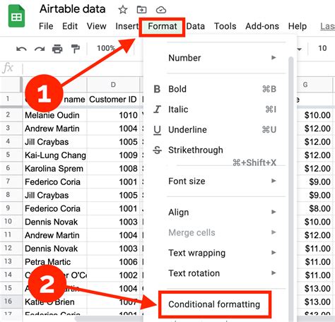
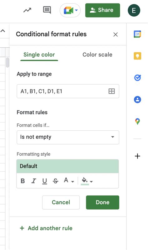
Conditional formatting is a feature that allows users to apply different formats to cells based on the values they contain. This can be useful for highlighting important information, such as cells that contain errors or cells that exceed a certain threshold. To apply conditional formatting in Google Sheets, users can select the cells they want to format, then go to the "Format" tab and select "Conditional formatting." From there, they can choose from a variety of pre-built rules or create their own custom rule using a formula.

One of the most common uses of conditional formatting is to highlight cells that contain a specific value. For example, users might want to highlight cells that contain the word "error" or cells that contain a specific date. However, there are also times when users need to highlight cells that do not contain a specific value. This is where the "does not equal" conditional formatting rule comes in.

How to Apply "Does Not Equal" Conditional Formatting in Google Sheets

To apply the "does not equal" conditional formatting rule in Google Sheets, users can follow these steps:

Select the cells they want to format.
Go to the "Format" tab and select "Conditional formatting."
In the formatting options panel, select "Custom formula is" from the drop-down menu.
Enter the formula =A1<> followed by the value they want to exclude.
Select the format they want to apply to the cells.
Click "Done" to apply the formatting.

For example, if users want to highlight all cells in column A that do not contain the word "error," they can enter the formula =A1<>"error" and select the format they want to apply.

Using the "Does Not Equal" Rule with Multiple Conditions

The "does not equal" conditional formatting rule can also be used with multiple conditions. For example, users might want to highlight cells that do not contain the word "error" and also do not contain the word "warning." To do this, they can enter the formula =AND(A1<>"error", A1<>"warning") and select the format they want to apply.

Here are some other examples of how to use the "does not equal" rule with multiple conditions:

=AND(A1<>"error", A1<>"warning", A1<>"info") - Highlights cells that do not contain the words "error," "warning," or "info."
=OR(A1<>"error", A1<>"warning") - Highlights cells that do not contain either the word "error" or the word "warning."
=NOT(OR(A1="error", A1="warning")) - Highlights cells that do not contain either the word "error" or the word "warning."

Common Use Cases for the "Does Not Equal" Rule

The "does not equal" conditional formatting rule has a wide range of use cases in Google Sheets. Here are some common examples:

Highlighting cells that do not contain a specific value, such as a product code or a customer name.
Identifying cells that do not meet a certain condition, such as cells that do not contain a specific date or cells that do not exceed a certain threshold.
Creating a to-do list or a task list, where cells that do not contain the word "done" are highlighted.
Analyzing data, where cells that do not contain a specific value or pattern are highlighted.

Best Practices for Using the "Does Not Equal" Rule

Here are some best practices for using the "does not equal" conditional formatting rule in Google Sheets:

Use the <> operator to specify the value that cells should not equal.
Use the AND and OR functions to combine multiple conditions.
Use the NOT function to negate a condition.
Test the formula before applying it to the entire range.
Use a clear and consistent naming convention for the formula.

By following these best practices, users can ensure that their conditional formatting rules are accurate and effective.

Tips and Tricks for Using Conditional Formatting in Google Sheets

Here are some tips and tricks for using conditional formatting in Google Sheets:

Use the "Format" tab to access the conditional formatting options.
Use the "Custom formula is" option to create a custom rule.
Use the =$ symbol to reference a cell or range.
Use the & symbol to concatenate text strings.
Use the TODAY() function to reference the current date.

By using these tips and tricks, users can create complex and powerful conditional formatting rules that help them analyze and visualize their data.

Common Errors to Avoid When Using Conditional Formatting

Here are some common errors to avoid when using conditional formatting in Google Sheets:

Using the wrong operator, such as = instead of <>.
Forgetting to include the = symbol at the beginning of the formula.
Using the wrong function, such as AND instead of OR.
Forgetting to test the formula before applying it to the entire range.
Using a formula that is too complex or nested.

By avoiding these common errors, users can ensure that their conditional formatting rules are accurate and effective.

Google Sheets Image Gallery

What is conditional formatting in Google Sheets?

Conditional formatting is a feature in Google Sheets that allows users to highlight cells based on specific conditions or criteria.

How do I apply the "does not equal" conditional formatting rule in Google Sheets?

To apply the "does not equal" conditional formatting rule, select the cells you want to format, go to the "Format" tab, select "Conditional formatting," and enter the formula `=A1<>` followed by the value you want to exclude.

What are some common use cases for the "does not equal" rule in Google Sheets?

The "does not equal" rule can be used to highlight cells that do not contain a specific value, identify cells that do not meet a certain condition, create a to-do list or task list, and analyze data.

In summary, the "does not equal" conditional formatting rule is a powerful tool in Google Sheets that allows users to highlight cells that do not contain a specific value. By following the steps outlined in this article, users can apply this rule to their data and gain valuable insights. Whether you're a beginner or an advanced user, the "does not equal" rule is an essential tool to have in your Google Sheets toolkit. So why not give it a try today and see the difference it can make in your data analysis and visualization? Share your experiences and tips with us in the comments below, and don't forget to share this article with your friends and colleagues who could benefit from learning about the "does not equal" rule in Google Sheets.