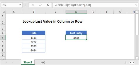
Intro
Getting the last value in a Google Sheets column can be useful for various tasks, such as tracking the latest entry in a dataset, calculating totals, or monitoring changes over time. There are several ways to achieve this, including using formulas, scripting, or even add-ons. Here, we'll focus on the most straightforward methods using formulas.
Using the OFFSET Function
The OFFSET function is one of the most common methods to get the last value in a column. It returns a range of cells that is a specified number of rows and columns away from a starting range.
=OFFSET(A1, COUNTA(A:A)-1, 0)
In this formula:
A1is the starting point. You can adjust this to any cell in the column you're interested in.COUNTA(A:A)-1calculates the number of cells in column A that contain data and then subtracts 1. This effectively gives us the position of the last cell with data relative to the starting point.0indicates that we're not moving horizontally (i.e., we stay in the same column).
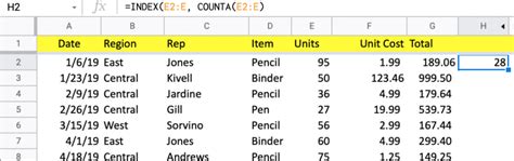
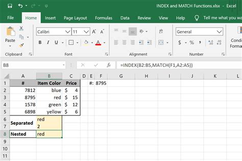
Using the INDEX and MATCH Functions
Another powerful combination for finding the last value is using INDEX and MATCH. This method is particularly useful because it's more flexible and can handle arrays more efficiently than OFFSET.
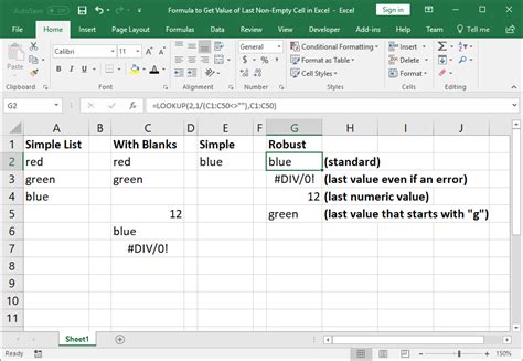
=INDEX(A:A, MATCH(2, 1/(A:A <> ""), 0))
In this formula:
A:Ais the range we're searching in.MATCH(2, 1/(A:A <> ""), 0)finds the relative position of the last non-empty cell in column A. Here's how it works:A:A <> ""creates an array ofTRUEandFALSEvalues indicating whether a cell is empty or not.1/(A:A <> "")converts theseTRUEandFALSEvalues into numbers (1 forTRUE, #DIV/0! forFALSE), becauseTRUEis treated as 1 andFALSEas 0 in math operations.MATCH(2,..., 0)looks for the second smallest number in this array, which corresponds to the last non-empty cell because all non-empty cells are represented by 1, and there's a virtual "2" at the end of the array (due to howMATCHworks with arrays).
INDEX(A:A,...)then returns the value at this position.
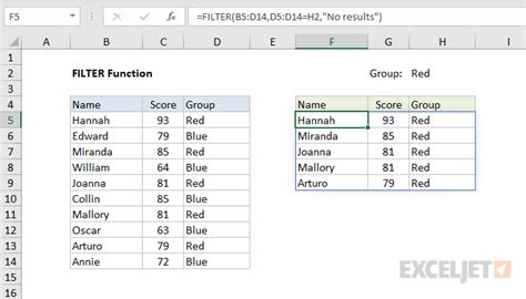
Using FILTER (Google Sheets)
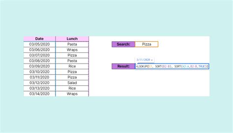
If you're using a version of Google Sheets that supports the FILTER function, you can also use it to get the last value in a column.
=FILTER(A:A, ROW(A:A) = MAX(ROW(A:A)*(A:A <> "")))
This formula filters column A to return only the cells that have a value and are in the last row that contains data. Here's how it works:
ROW(A:A)*(A:A <> "")creates an array where each non-empty cell's row number is preserved, and empty cells result in a 0 (becauseFALSEis treated as 0).MAX(...)finds the maximum row number in this array, which corresponds to the last non-empty cell.FILTER(A:A,...)then returns the value in column A for this maximum row number.
Choosing the Right Method
Each of these methods has its use cases. The OFFSET and INDEX/MATCH combinations are quite versatile and work well in most situations. The FILTER function is a more modern approach and can be useful, especially when working with larger datasets or when you need to perform more complex filtering.
Regardless of the method you choose, these formulas provide powerful tools for dynamically accessing the last value in a Google Sheets column, making it easier to monitor and analyze your data.

Practical Applications
These formulas can be applied in various scenarios, such as:
- Automating Reports: Use the last value in a column to automatically update reports or summaries.
- Tracking Changes: Monitor the last entry in a dataset to track changes or updates over time.
- Data Analysis: Use the last value as part of a larger analysis, such as calculating averages or totals based on the most recent data.
Step-by-Step Guide
For those who are new to using formulas in Google Sheets, here's a step-by-step guide to getting started:
- Select the Cell: Choose where you want the last value to appear.
- Enter the Formula: Type in the formula you've chosen, adjusting the column letters as necessary.
- Press Enter: The formula will calculate, and the last value will appear.
- Adjust as Needed: If your data changes, the formula will automatically update to show the new last value.

Tips and Variations
- Handling Errors: If your column might contain errors, consider wrapping your formula in an
IFERRORfunction to return a custom message instead. - Dynamic Ranges: Use named ranges or the
OFFSETfunction to create dynamic ranges that adjust as your data grows. - Multiple Columns: If you need to get the last value from multiple columns, you can adjust the column letters in your formula or use an array formula.
Common Issues
- #REF! Errors: These often occur if the formula references a range that doesn't exist. Check your column letters and range sizes.
- #VALUE! Errors: These can happen if the formula is trying to perform an operation on a value of the wrong type. Ensure your data is consistent.
Advanced Techniques
For more complex scenarios, consider using Google Sheets' scripting capabilities or exploring add-ons that can automate tasks based on the last value in a column.

Best Practices
- Keep it Simple: Unless necessary, avoid complex formulas that can be hard to understand and maintain.
- Test Thoroughly: Always test your formulas with different scenarios to ensure they work as expected.
- Document Your Work: Leave comments or notes explaining what your formulas do, especially in shared worksheets.
Last Value Image Gallery


How do I get the last value in a Google Sheets column?
+You can use formulas like OFFSET, INDEX/MATCH, or FILTER to get the last value in a column. The choice of formula depends on your specific needs and the structure of your data.
What is the OFFSET function used for?
+The OFFSET function is used to return a range of cells that is a specified number of rows and columns away from a starting range. It's useful for getting the last value in a column when you know the starting point.
How does the INDEX/MATCH function combination work?
+The INDEX/MATCH combination is a powerful way to look up values in Google Sheets. INDEX returns a value at a specified position in a range, while MATCH finds the relative position of a value within a range. Together, they can be used to find the last value in a column by matching the last occurrence of a non-empty cell.
If you've made it this far, you're likely eager to start using these formulas to get the last value in your Google Sheets columns. Whether you're automating reports, tracking changes, or simply need to analyze the most recent data, these methods provide flexible and powerful solutions. Feel free to share your experiences or ask further questions in the comments below. Don't forget to share this article with anyone who might find it useful, and consider bookmarking it for future reference. Happy spreadsheeting!