Intro
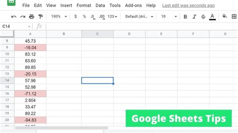
Learn how to display Google Sheets negative numbers in red, using custom number formatting and conditional formatting rules to highlight negative values, percentages, and currencies for better data visualization and financial analysis.
The world of Google Sheets can be a powerful tool for managing and analyzing data, but it can also be frustrating when dealing with negative numbers. Negative numbers can be particularly problematic when trying to format them in a way that stands out, such as displaying them in red. In this article, we will delve into the importance of formatting negative numbers in Google Sheets, the benefits of doing so, and provide a step-by-step guide on how to display negative numbers in red.
Formatting negative numbers in Google Sheets is crucial for financial analysis, accounting, and other fields where negative numbers can have significant implications. By displaying negative numbers in red, users can quickly and easily identify areas where they may be losing money or experiencing a deficit. This can help users make informed decisions and take corrective action to mitigate losses. Moreover, formatting negative numbers in red can also help users to distinguish between positive and negative numbers, reducing the risk of errors and misinterpretations.
In addition to its practical applications, formatting negative numbers in Google Sheets can also be useful for creating visually appealing and easy-to-understand reports and dashboards. By using conditional formatting to display negative numbers in red, users can create a clear and concise visual representation of their data, making it easier to communicate insights and trends to stakeholders. This can be particularly useful for business owners, financial analysts, and other professionals who need to present complex data to non-technical audiences.
Why Format Negative Numbers in Google Sheets?
Formatting negative numbers in Google Sheets can have numerous benefits, including improved data visualization, enhanced decision-making, and increased productivity. By displaying negative numbers in red, users can quickly identify areas where they need to focus their attention, making it easier to prioritize tasks and allocate resources. Additionally, formatting negative numbers in red can also help users to detect errors and inconsistencies in their data, reducing the risk of mistakes and misinterpretations.
Benefits of Formatting Negative Numbers in Google Sheets
- Improved data visualization: Formatting negative numbers in red can help users to quickly and easily identify areas where they may be losing money or experiencing a deficit.
- Enhanced decision-making: By displaying negative numbers in red, users can make informed decisions and take corrective action to mitigate losses.
- Increased productivity: Formatting negative numbers in red can help users to prioritize tasks and allocate resources more effectively, reducing the time and effort required to analyze and interpret data.
How to Format Negative Numbers in Google Sheets
Formatting negative numbers in Google Sheets is a relatively straightforward process that can be accomplished using conditional formatting. Here's a step-by-step guide on how to do it:
- Select the cells that you want to format: To format negative numbers in Google Sheets, you need to select the cells that contain the numbers you want to format.
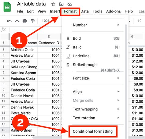
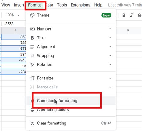
- Go to the "Format" tab: Once you've selected the cells, go to the "Format" tab in the top menu.
- Select "Conditional formatting": From the "Format" tab, select "Conditional formatting" from the drop-down menu.
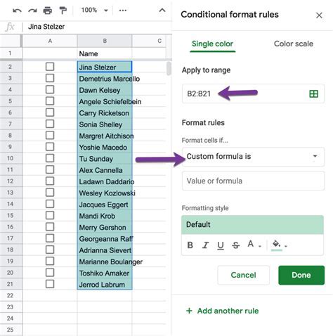
- Set up the formatting rule: In the conditional formatting panel, set up a formatting rule that says "Format cells if" and select "Custom formula is" from the drop-down menu.
- Enter the formula: Enter the formula
=A1<0, where A1 is the cell that you want to format. This formula will apply the formatting to any cell that contains a negative number. - Select the formatting options: Once you've entered the formula, select the formatting options that you want to apply to the negative numbers, such as font color, background color, and number formatting.
- Click "Done": Finally, click "Done" to apply the formatting rule to the selected cells.
Step-by-Step Guide to Formatting Negative Numbers in Google Sheets
- Select the cells that you want to format
- Go to the "Format" tab
- Select "Conditional formatting"
- Set up the formatting rule
- Enter the formula
=A1<0 - Select the formatting options
- Click "Done"
Common Issues with Formatting Negative Numbers in Google Sheets
While formatting negative numbers in Google Sheets can be a powerful tool for data analysis and visualization, there are some common issues that users may encounter. Here are some of the most common issues and how to troubleshoot them:
- Inconsistent formatting: If the formatting is not applying consistently to all cells, check that the formula is correct and that the formatting options are set up correctly.
- Errors in the formula: If the formula is not working correctly, check that it is entered correctly and that there are no errors in the formula.
- Conflicting formatting rules: If there are conflicting formatting rules, try to simplify the rules or use a different approach to formatting the negative numbers.
Troubleshooting Common Issues with Formatting Negative Numbers in Google Sheets
- Check the formula for errors
- Check the formatting options for consistency
- Simplify conflicting formatting rules
- Use a different approach to formatting the negative numbers
Best Practices for Formatting Negative Numbers in Google Sheets
To get the most out of formatting negative numbers in Google Sheets, here are some best practices to follow:
- Use consistent formatting: Use consistent formatting throughout the spreadsheet to make it easier to read and understand.
- Use clear and concise labels: Use clear and concise labels to make it easier to identify what the data represents.
- Avoid using too many formatting rules: Avoid using too many formatting rules, as this can make the spreadsheet difficult to read and understand.
- Use conditional formatting: Use conditional formatting to apply formatting rules to specific cells or ranges of cells.
Best Practices for Formatting Negative Numbers in Google Sheets
- Use consistent formatting
- Use clear and concise labels
- Avoid using too many formatting rules
- Use conditional formatting
Google Sheets Image Gallery


How do I format negative numbers in Google Sheets?
+To format negative numbers in Google Sheets, select the cells that you want to format, go to the "Format" tab, select "Conditional formatting", and set up a formatting rule that says "Format cells if" and select "Custom formula is" from the drop-down menu. Enter the formula `=A1<0`, where A1 is the cell that you want to format, and select the formatting options that you want to apply to the negative numbers.
What are the benefits of formatting negative numbers in Google Sheets?
+The benefits of formatting negative numbers in Google Sheets include improved data visualization, enhanced decision-making, and increased productivity. By displaying negative numbers in red, users can quickly and easily identify areas where they may be losing money or experiencing a deficit, making it easier to prioritize tasks and allocate resources.
How do I troubleshoot common issues with formatting negative numbers in Google Sheets?
+To troubleshoot common issues with formatting negative numbers in Google Sheets, check the formula for errors, check the formatting options for consistency, simplify conflicting formatting rules, and use a different approach to formatting the negative numbers. If the issue persists, try seeking help from a Google Sheets expert or searching for solutions online.
In final thoughts, formatting negative numbers in Google Sheets can be a powerful tool for data analysis and visualization. By following the steps outlined in this article, users can quickly and easily format negative numbers in red, making it easier to identify areas where they may be losing money or experiencing a deficit. Whether you're a business owner, financial analyst, or simply a Google Sheets user, formatting negative numbers in red can help you make informed decisions and take corrective action to mitigate losses. So why not give it a try today and see the difference it can make for yourself? Share your thoughts and experiences with formatting negative numbers in Google Sheets in the comments below, and don't forget to share this article with your friends and colleagues who may benefit from it.