Google Sheets Sumif Multiple Criteria

The ability to sum values based on multiple criteria in Google Sheets is a powerful feature that can help users analyze and understand their data more effectively. This functionality is often required in various data analysis tasks, such as financial reporting, inventory management, and more. The SUMIF function in Google Sheets allows users to sum values in a specified range based on a single condition, but when it comes to multiple criteria, the SUMIFS function is the more appropriate tool.

The SUMIFS function in Google Sheets is designed to sum values in a specified range based on multiple conditions. It provides a flexible and efficient way to analyze data by applying multiple filters. This function is particularly useful when working with large datasets where the need to apply multiple criteria to narrow down data is common.

Introduction to SUMIFS

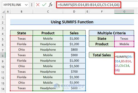
The SUMIFS function is an extension of the SUMIF function, with the key difference being its ability to apply multiple criteria across different ranges. The syntax of the SUMIFS function is as follows:

SUMIFS(sum_range, criteria_range1, criteria1, [criteria_range2], [criteria2],...)

sum_range: The range of cells that you want to sum.
criteria_range1: The range of cells that you want to apply the first criteria against.
criteria1: The first criteria that you want to apply.
[criteria_range2], [criteria2], etc.: Optional additional ranges and criteria to apply.

How to Use SUMIFS

To effectively use the SUMIFS function, follow these steps:

Identify Your Data: First, ensure your data is organized in a way that makes it easy to apply criteria. Typically, this means having your data in a table format with headers in the first row.
Select Your Sum Range: Determine which column contains the values you want to sum. This will be your sum_range.
Determine Your Criteria Ranges and Criteria: Identify the columns and the specific values within those columns that you want to use as your criteria. These will be your criteria_range1, criteria1, etc.
Apply the SUMIFS Function: In a new cell where you want the sum to appear, start typing =SUMIFS(, then select your sum_range, followed by your first criteria_range and criteria, and so on. You can add as many criteria ranges and criteria as needed.
Close the Function: After entering all your ranges and criteria, close the function with a parenthesis ) and press Enter to execute the function.

Examples of Using SUMIFS

Example 1: Summing Sales by Region and Product

Suppose you have a sales dataset with columns for Sales Amount, Region, and Product, and you want to sum the sales amount for a specific region and product.

Sales Amount	Region	Product
100	North	A
200	North	B
50	South	A
150	South	B

If you want to sum the sales amount for the North region and product A, your SUMIFS formula might look like this:

=SUMIFS(A2:A5, B2:B5, "North", C2:C5, "A")

Example 2: Summing Expenses by Category and Date

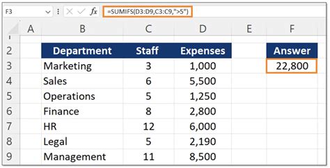
If you have an expenses dataset with columns for Expense Amount, Category, and Date, and you want to sum the expense amount for a specific category and date range.

Expense Amount	Category	Date
50	Food	2023-01-01
100	Transport	2023-01-02
75	Food	2023-01-03
200	Transport	2023-01-04

To sum the expense amount for the Food category and dates after 2023-01-01, your SUMIFS formula might look like this:

=SUMIFS(A2:A5, B2:B5, "Food", C2:C5, ">2023-01-01")

Tips and Tricks

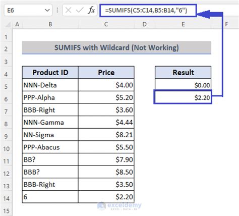
Using Wildcards: In your criteria, you can use wildcards like * (asterisk) to match any sequence of characters and ? (question mark) to match a single character. For example, =SUMIFS(A2:A5, B2:B5, "N*") sums values where the region starts with "N".
Using Dates: When working with dates, ensure your criteria are in a format that Google Sheets recognizes as dates. You can use the DATE function or directly input dates in a recognized format.
Handling Errors: If your SUMIFS function returns an error, check that your ranges and criteria are correctly formatted and that there are no typos in your formula.

Advanced SUMIFS Techniques

For more complex data analysis, understanding how to combine SUMIFS with other Google Sheets functions can be incredibly powerful. This might include using SUMIFS in conjunction with the IF function for conditional logic, or with the INDEX and MATCH functions for more dynamic range selections.

Combining SUMIFS with IF

The IF function can be used within the criteria of a SUMIFS function to apply conditional logic. For example, to sum values where a certain condition is true, you might use a formula like:

=SUMIFS(A2:A5, IF(B2:B5="Condition", "Yes", "No"), "Yes")

However, this approach is less common and usually, the IF function is used outside the SUMIFS to control the criteria based on other conditions.

Using SUMIFS with INDEX and MATCH

The INDEX and MATCH functions can be used to create dynamic criteria ranges or to sum ranges based on criteria that are determined by other parts of your spreadsheet.

=SUMIFS(INDEX(A:A, MATCH("Header", A1:A5, 0)), B:B, "Criteria")

This approach allows for more flexibility, especially in reports where the structure might change over time.

Common Errors and Troubleshooting

When working with the SUMIFS function, several common errors can occur. These include:

#N/A Error: This error often occurs when the criteria range and criteria do not match any cells in the range. Ensure that your criteria are correctly spelled and formatted.
#VALUE! Error: This can happen if the sum range contains non-numeric values. Make sure your sum range only includes numbers or cells that can be coerced into numbers.
Incorrect Sum: Double-check that your criteria ranges and sum range are correctly aligned and that you have not missed any criteria.

To troubleshoot, start by breaking down your formula into smaller parts to identify where the error is occurring. Use the EVALUATE FORMULA feature in Google Sheets to step through your formula and see the results of each part.

Best Practices

Keep It Simple: While the SUMIFS function can handle multiple criteria, try to keep your formulas as simple as possible to avoid confusion.
Use References: Instead of hard-coding criteria into your formula, use cell references. This makes your formulas more dynamic and easier to update.
Test Your Formula: Always test your SUMIFS formula with known data to ensure it is working as expected before applying it to larger datasets.

Alternatives to SUMIFS

While SUMIFS is a powerful function, there are scenarios where alternative approaches might be more suitable. These include:

Using Pivot Tables: Pivot tables can sum values based on multiple criteria and offer a more visual and interactive way to analyze data.
Using FILTER: The FILTER function can be used to sum values that meet certain criteria, offering a more flexible and powerful alternative to SUMIFS in some cases.
Using QUERY: The QUERY function allows you to perform SQL-like queries on your data, including summing values based on multiple criteria.

Each of these alternatives has its own strengths and can be chosen based on the specific requirements of your data analysis task.

Pivot Tables

Pivot tables are a great way to summarize large datasets and can easily sum values based on multiple criteria. They offer the advantage of being highly interactive, allowing users to quickly change the criteria and see the results.

Using FILTER

The FILTER function can be used in combination with the SUM function to achieve results similar to SUMIFS. It is particularly useful when you need to apply complex criteria that involve logical operations.

=SUM(FILTER(A2:A5, (B2:B5="North") * (C2:C5="A")))

Using QUERY

The QUERY function provides a SQL-like interface to your data, allowing you to select, filter, and aggregate data in a very flexible way.

=QUERY(A2:C5, "SELECT SUM(A) WHERE B = 'North' AND C = 'A'")

Google Sheets SUMIFS Gallery

What is the difference between SUMIF and SUMIFS?

The main difference is that SUMIF can only apply one condition, while SUMIFS can apply multiple conditions across different ranges.

How do I use wildcards in SUMIFS criteria?

You can use `*` to match any sequence of characters and `?` to match a single character. For example, `=SUMIFS(A2:A5, B2:B5, "N*")` sums values where the region starts with "N".

Can I use SUMIFS with dates?

Yes, you can use SUMIFS with dates. Ensure your criteria are in a format that Google Sheets recognizes as dates. You can use the `DATE` function or directly input dates in a recognized format.

As you continue to explore the capabilities of the SUMIFS function and other related functions in Google Sheets, remember that practice makes perfect. Experimenting with different scenarios and datasets will help solidify your understanding and make you more proficient in data analysis tasks. If you have any questions or need further clarification on any of the topics discussed, feel free to ask in the comments below. Share this article with anyone who might benefit from learning about the SUMIFS function and its applications in Google Sheets.