Google Sheets Sumif Multiple Criteria

The world of spreadsheet analysis is a vast and wondrous place, full of formulas and functions that can help you unlock the secrets of your data. One of the most powerful tools in your arsenal is the SUMIF function, which allows you to sum up values in a range based on a single criteria. But what if you need to sum up values based on multiple criteria? That's where the SUMIFS function comes in.

In this article, we'll explore the ins and outs of using SUMIFS in Google Sheets to sum up values based on multiple criteria. We'll cover the basics of the function, including its syntax and how to use it, as well as some more advanced techniques for using SUMIFS to analyze your data.

Introduction to SUMIFS

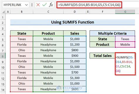
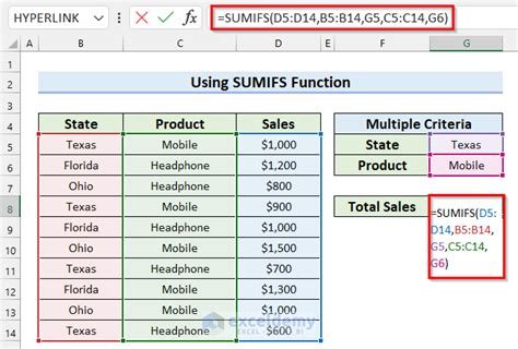
The SUMIFS function is a variation of the SUMIF function that allows you to sum up values in a range based on multiple criteria. The syntax for the SUMIFS function is as follows:

SUMIFS(sum_range, criteria_range1, criteria1, [criteria_range2], [criteria2],...)

Where:

sum_range is the range of cells that you want to sum up
criteria_range1 is the range of cells that you want to apply the first criteria to
criteria1 is the first criteria that you want to apply
[criteria_range2] and [criteria2] are optional additional criteria that you can apply

How to Use SUMIFS

To use the SUMIFS function, you'll need to follow these steps:

Select the cell where you want to display the sum
Type in the formula =SUMIFS(
Select the range of cells that you want to sum up (sum_range)
Select the range of cells that you want to apply the first criteria to (criteria_range1)
Enter the first criteria (criteria1)
If you want to apply additional criteria, select the range of cells that you want to apply the next criteria to (criteria_range2) and enter the next criteria (criteria2)
Repeat steps 6 until you've applied all of the criteria that you want to use
Close the formula with a )

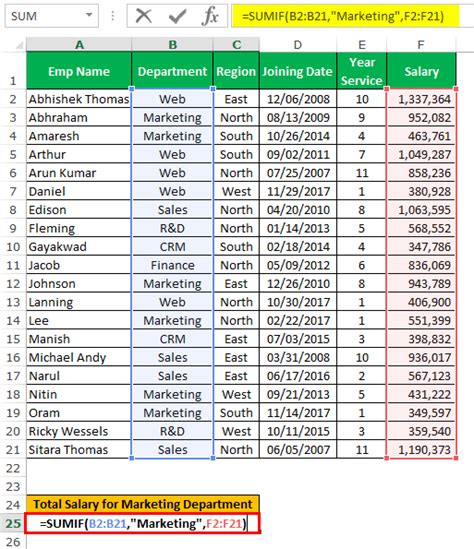
For example, suppose you have a range of sales data that includes the date, region, and amount of each sale. You can use the SUMIFS function to sum up the total amount of sales for a specific region and date range. The formula might look like this:

=SUMIFS(B:B, A:A, "North", C:C, ">="&DATE(2022,1,1), C:C, "<="&DATE(2022,12,31))

This formula sums up the values in column B (the sales amounts) for the rows where the value in column A (the region) is "North" and the value in column C (the date) is between January 1, 2022 and December 31, 2022.

Advanced Techniques for Using SUMIFS

While the basic syntax for the SUMIFS function is straightforward, there are some advanced techniques that you can use to get more out of the function.

One of the most powerful techniques is to use wildcards in your criteria. For example, if you want to sum up the total amount of sales for all regions that start with the letter "N", you can use the formula:

=SUMIFS(B:B, A:A, "N*")

This formula sums up the values in column B for the rows where the value in column A starts with the letter "N".

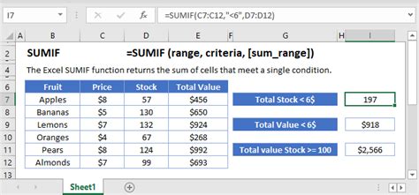
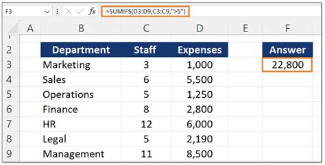
Another technique is to use the SUMIFS function in combination with other functions, such as the IF function. For example, if you want to sum up the total amount of sales for a specific region, but only if the sales amount is greater than a certain threshold, you can use the formula:

=SUMIFS(B:B, A:A, "North", B:B, ">100")

This formula sums up the values in column B for the rows where the value in column A is "North" and the value in column B is greater than 100.

Common Errors to Avoid

When using the SUMIFS function, there are a few common errors to avoid.

One of the most common errors is to forget to close the formula with a ). This can cause the formula to return an error message, rather than the correct result.

Another common error is to enter the criteria incorrectly. For example, if you want to sum up the total amount of sales for a specific region, you'll need to enter the region name exactly as it appears in the data. If you enter the region name incorrectly, the formula will return an error message.

To avoid these errors, it's a good idea to double-check your formula before you enter it. You can also use the formula auditing tools in Google Sheets to help you identify and fix errors.

Best Practices for Using SUMIFS

To get the most out of the SUMIFS function, there are a few best practices to keep in mind.

One of the most important best practices is to use clear and concise criteria. This will help you avoid errors and ensure that your formula returns the correct result.

Another best practice is to use the SUMIFS function in combination with other functions, such as the IF function. This will allow you to create more complex and powerful formulas that can help you analyze your data in new and interesting ways.

Finally, it's a good idea to use the formula auditing tools in Google Sheets to help you identify and fix errors. These tools can help you ensure that your formula is correct and that it's returning the correct result.

Real-World Examples of Using SUMIFS

The SUMIFS function is a powerful tool that can be used in a wide range of real-world scenarios.

For example, suppose you're a sales manager and you want to sum up the total amount of sales for a specific region and date range. You can use the SUMIFS function to create a formula that sums up the values in the sales column for the rows where the region is "North" and the date is between January 1, 2022 and December 31, 2022.

Another example is a marketing manager who wants to sum up the total amount of revenue generated by a specific campaign. You can use the SUMIFS function to create a formula that sums up the values in the revenue column for the rows where the campaign name is "Campaign A" and the date is between January 1, 2022 and December 31, 2022.

Google Sheets SUMIFS Image Gallery

What is the SUMIFS function in Google Sheets?

The SUMIFS function is a variation of the SUMIF function that allows you to sum up values in a range based on multiple criteria.

How do I use the SUMIFS function in Google Sheets?

To use the SUMIFS function, select the cell where you want to display the sum, type in the formula =SUMIFS(, select the range of cells that you want to sum up, select the range of cells that you want to apply the first criteria to, enter the first criteria, and repeat the process for each additional criteria.

What are some common errors to avoid when using the SUMIFS function?

Common errors to avoid when using the SUMIFS function include forgetting to close the formula with a ) and entering the criteria incorrectly.

What are some best practices for using the SUMIFS function?

Best practices for using the SUMIFS function include using clear and concise criteria, using the function in combination with other functions, and using the formula auditing tools in Google Sheets to help identify and fix errors.

Can I use the SUMIFS function with other Google Sheets functions?

Yes, you can use the SUMIFS function with other Google Sheets functions, such as the IF function, to create more complex and powerful formulas.

In conclusion, the SUMIFS function is a powerful tool that can help you analyze your data in new and interesting ways. By following the best practices outlined in this article and avoiding common errors, you can get the most out of the SUMIFS function and take your data analysis to the next level. We encourage you to share your own experiences with using the SUMIFS function in the comments below, and to ask any questions you may have about how to use the function. Additionally, if you found this article helpful, please consider sharing it with others who may benefit from learning about the SUMIFS function.