Excel Freeze Two Rows

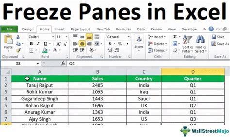
Freezing rows in Excel is a useful feature that allows you to keep certain rows visible while scrolling through your worksheet. This can be particularly helpful when working with large datasets where you need to keep headers or other important information in view at all times. Freezing two rows in Excel is a straightforward process that can be accomplished in a few steps.

To begin with, it's essential to understand why freezing rows is beneficial. In many cases, when you're working with a large spreadsheet, you might find yourself scrolling down to view data, but you also need to keep the header row or other critical information visible. This is where the freeze feature comes into play. It allows you to lock specific rows at the top of your worksheet, ensuring they remain visible regardless of how far you scroll down.

Understanding Excel's Freeze Feature

Excel offers several options for freezing panes, including freezing the top row, freezing the first column, or freezing both. The process for freezing two rows is similar to freezing any other number of rows, with the main difference being the selection of the rows you wish to freeze.

Steps to Freeze Two Rows in Excel

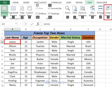
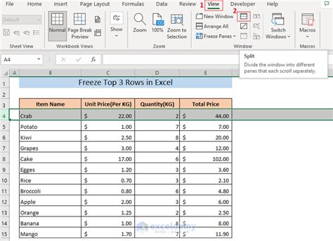
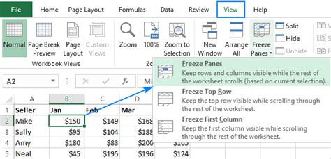
Select the Row Below the Rows You Want to Freeze: To freeze the first two rows, you need to select the third row. This is because Excel freezes all rows above the selected row. So, if you want to freeze rows 1 and 2, you should select row 3.
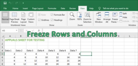
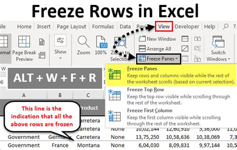
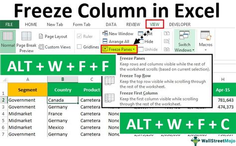
Go to the View Tab: In the ribbon at the top of Excel, click on the "View" tab. This tab contains various options for viewing your worksheet, including the freeze panes feature.
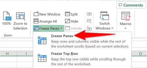
Click on Freeze Panes: Within the "View" tab, find the "Window" group, and click on "Freeze Panes." A dropdown menu will appear with options to freeze the top row, freeze the first column, or freeze panes.
Select Freeze Panes: From the dropdown menu, select "Freeze Panes." This option allows you to freeze both rows and columns. Since you've selected the row below the ones you want to freeze, Excel will lock all rows above your selection.
Verify the Freeze: After you've frozen the panes, you should see a gray line indicating where the freeze is applied. You can now scroll down through your worksheet, and the first two rows will remain visible.

Alternative Method: Using the Freeze Top Row Option

If you only need to freeze the very top row, Excel provides a quicker method:

Select the Cell Below the Row You Want to Freeze: If you want to freeze just the first row, select any cell in the second row.
Go to the View Tab and Click on Freeze Top Row: In the "View" tab, find the "Window" group, and click on "Freeze Panes" > "Freeze Top Row."

This method is more direct but is limited to freezing only the top row.

Tips and Variations

Freezing Columns: You can also freeze columns by selecting the column to the right of the one you want to freeze and then using the "Freeze Panes" option.
Unfreezing Panes: If you need to unfreeze your panes, go to the "View" tab, click on "Freeze Panes," and select "Unfreeze Panes."
Using Freeze Panes for Complex Worksheets: For more complex worksheets where you need to freeze both rows and columns, select the cell below the row you want to freeze and to the right of the column you want to freeze, then use the "Freeze Panes" option.

Benefits of Freezing Rows

Freezing rows in Excel offers several benefits, including:

Improved readability by keeping headers visible.
Enhanced productivity by reducing the need to scroll up to view important information.
Better data analysis by allowing you to view context (like headers) while scrolling through data.

Common Issues and Solutions

Sometimes, you might encounter issues with freezing panes, such as:

Inability to Freeze Panes: Ensure you're selecting the correct row or column and that you're using the "Freeze Panes" option correctly.
Frozen Panes Not Working as Expected: Check if your selection is correct and if you've applied the freeze correctly.

Best Practices for Using Freeze Panes

Use Freeze Panes Judiciously: Only freeze the rows and columns that are necessary, as excessive use can clutter your worksheet.
Combine with Other Viewing Options: Experiment with combining freeze panes with other viewing options, like zooming or using multiple windows, to optimize your workflow.

Excel Freeze Rows Image Gallery

How do I freeze two rows in Excel?

To freeze two rows, select the third row, go to the "View" tab, click on "Freeze Panes," and then select "Freeze Panes" from the dropdown menu.

Can I freeze both rows and columns in Excel?

Yes, you can freeze both rows and columns. To do this, select the cell below the row you want to freeze and to the right of the column you want to freeze, then use the "Freeze Panes" option.

How do I unfreeze panes in Excel?

To unfreeze panes, go to the "View" tab, click on "Freeze Panes," and then select "Unfreeze Panes" from the dropdown menu.

In conclusion, freezing two rows in Excel is a simple yet powerful feature that can significantly improve your productivity and data analysis capabilities. By following the steps and tips outlined in this article, you can master the use of freeze panes and take your Excel skills to the next level. Whether you're working with small datasets or large, complex spreadsheets, the ability to freeze rows and columns will prove to be an invaluable tool in your Excel toolkit. So, the next time you find yourself scrolling through a lengthy spreadsheet, remember the convenience and efficiency that freezing rows can offer, and make the most out of this feature to enhance your Excel experience.