Add Benchmark Line In Excel Graph

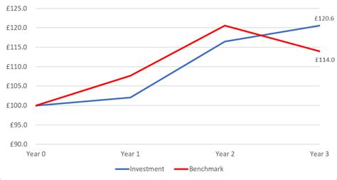
When working with data in Excel, adding a benchmark line to a graph can be incredibly useful for comparing performance, tracking progress, or setting targets. A benchmark line provides a visual reference point, making it easier to understand how actual data points relate to a specific standard or goal. Here's how you can add a benchmark line to an Excel graph, along with explanations and examples to guide you through the process.

To start, let's consider the importance of visualizing data. Data visualization is a powerful tool for communicating information, and Excel offers a wide range of options for creating graphs and charts. By adding a benchmark line, you can enhance your graphs and make them more informative.

Understanding Benchmark Lines

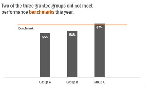
Benchmark lines are horizontal or vertical lines on a chart that represent a target value, average, or any other significant data point that you want to highlight. They can be particularly useful in line charts, column charts, and area charts where you're tracking data over time or across categories.

Adding a Benchmark Line to an Excel Graph

To add a benchmark line, follow these steps:

Prepare Your Data: Ensure your data is organized in a table format with headers. This will make it easier to create and manipulate your chart.
Create a Chart: Select your data range, including headers, and go to the "Insert" tab in the ribbon. Choose the type of chart you want (e.g., line chart, column chart) from the "Charts" group.
Add a Benchmark Line:
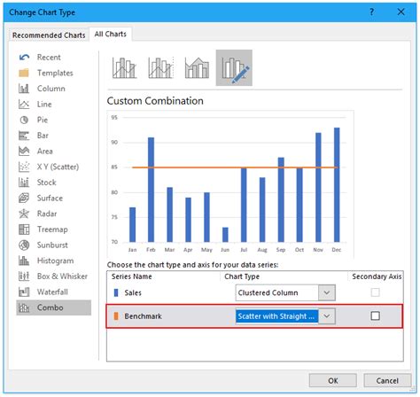
- Method 1: Using a Secondary Axis:
  - Add a new series to your chart that represents your benchmark value. This can be a constant value or a formula that calculates the benchmark.
  - Right-click on the new series in the chart and select "Format Data Series."
  - Choose to plot the series on a secondary axis.
  - Format the series as a line and adjust its appearance as needed.
- Method 2: Using a Horizontal/Vertical Line:
  - Go to the "Chart Tools" tab in the ribbon.
  - Click on "Trendline" in the "Analysis" group.
  - Select "Horizontal Line" or "Vertical Line" and then choose "Constant."
  - Enter the value for your benchmark line.

Customizing Your Benchmark Line

After adding a benchmark line, you can customize its appearance to make it stand out or blend in with your chart, depending on your needs. Here are a few tips:

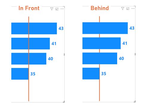
Color and Line Style: Change the color and line style of your benchmark line to differentiate it from other data series. Right-click on the line and select "Format Data Series" to access these options.
Line Width: Adjust the line width to make the benchmark line more or less prominent.
Markers: If your benchmark line intersects with data points, consider adding markers to highlight these intersections.

Practical Applications of Benchmark Lines

Benchmark lines have a wide range of practical applications across different industries and fields. Here are a few examples:

Sales Performance: Use a benchmark line to represent a sales target. Actual sales data can then be compared against this target to assess performance.
Quality Control: In manufacturing, benchmark lines can represent quality standards. Data points below the benchmark line might indicate a need for improvement.
Financial Analysis: Benchmark lines can be used to track stock prices against a moving average or to compare budgeted expenses versus actual expenses.

Benefits of Using Benchmark Lines

The benefits of using benchmark lines in Excel graphs include:

Enhanced Visualization: Benchmark lines make graphs more informative by providing a clear point of reference.
Improved Analysis: They facilitate more accurate and meaningful analysis by allowing for easy comparison of actual data against targets or standards.
Better Decision Making: By clearly visualizing how data points relate to benchmarks, decision-makers can identify trends, opportunities, and challenges more effectively.

Benchmark Line Image Gallery

How do I add a benchmark line in Excel?

To add a benchmark line, you can either use a secondary axis for a new data series representing your benchmark or add a horizontal/vertical line through the trendline option in the Chart Tools tab.

What are the benefits of using benchmark lines in Excel graphs?

Benchmark lines enhance visualization, improve analysis by providing a clear reference point, and facilitate better decision-making by highlighting how data points compare to targets or standards.

Can I customize the appearance of a benchmark line in Excel?

Yes, you can customize the color, line style, and width of a benchmark line, as well as add markers, to make it more distinguishable and effective in your graph.

In conclusion, adding a benchmark line to an Excel graph is a straightforward process that can significantly enhance the utility and clarity of your data visualizations. By following the steps and tips outlined above, you can effectively use benchmark lines to support your analysis, presentation, and decision-making processes. Whether you're working in sales, finance, quality control, or any other field, benchmark lines can provide valuable insights and help you achieve your goals. Feel free to share your experiences or ask questions about using benchmark lines in Excel, and don't forget to explore other features and functions that Excel has to offer to take your data analysis to the next level.