How To Change Excel Cell Color Based On Text

Changing the color of cells in Excel based on the text they contain can be a useful way to highlight important information, differentiate between various types of data, and make your spreadsheets more visually appealing. Excel provides several methods to achieve this, including using Conditional Formatting, a powerful tool that allows you to apply formatting to cells based on specific conditions. Here, we'll explore how to change Excel cell color based on text using Conditional Formatting and other methods.

Excel's Conditional Formatting feature is intuitive and offers a lot of flexibility. It allows you to format cells based on their values, formulas, or formatting. To change cell color based on text, you can use the "Text Contains" or "Equal to" options within Conditional Formatting. Let's dive into how to do it.

Introduction to Conditional Formatting

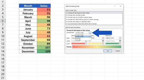
Conditional Formatting in Excel is a feature that allows you to format cells based on the values of those cells. You can apply several types of formatting, including changing the fill color, font color, and more, based on conditions you specify. The conditions can range from simple comparisons (like "greater than" or "less than") to more complex formulas.

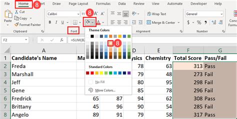
To access Conditional Formatting, select the cells you want to format, go to the "Home" tab on the Excel ribbon, and find the "Styles" group. Click on "Conditional Formatting" to open the menu and choose the type of formatting rule you want to apply.

Applying Conditional Formatting to Change Cell Color Based on Text

To change the cell color based on text, follow these steps:

Select the Cells: Choose the range of cells you want to apply the formatting to.
Go to Conditional Formatting: On the "Home" tab, click on "Conditional Formatting" in the "Styles" group.
New Rule: Select "New Rule" to open the New Formatting Rule dialog box.
Use a Formula: Choose "Use a formula to determine which cells to format."
Enter the Formula: In the formula box, you can enter a formula like =A1="Specific Text" if you want to highlight cells that contain the exact phrase "Specific Text." For cells that contain specific text anywhere within them, you can use =ISNUMBER(SEARCH("text",A1)).
Format: Click on the "Format" button to choose how you want to format the cells that meet the condition, such as changing the fill color.
Apply: Click "OK" to apply the rule.

For example, to highlight all cells in column A that contain the word "example," you would use the formula =ISNUMBER(SEARCH("example",A1)) and then select a fill color.

Using the "Text Contains" Rule

Excel also provides a more straightforward "Text Contains" rule that can be accessed directly from the Conditional Formatting menu:

Select the Cells: Choose the range of cells.
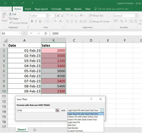
Conditional Formatting: Go to "Conditional Formatting" > "Highlight Cells Rules" > "Text Contains."
Specify the Text: In the dialog box, enter the text you're looking for.
Choose a Format: Select the formatting you want to apply.
OK: Click "OK" to apply the rule.

This method is quicker for simple text searches but might not offer the flexibility of using a formula.

Formatting Cells Based on the Value of Another Cell

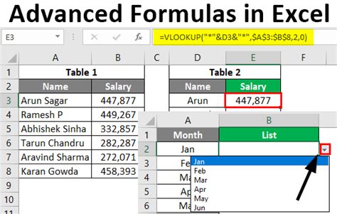
Sometimes, you might want to change the color of a cell based on the value of another cell. This can be achieved by using a formula within Conditional Formatting. For instance, if you want to highlight cell B1 based on the value in cell A1, you could use a rule like =A1="Specific Text" and apply it to cell B1.

Practical Applications

Changing cell color based on text has numerous practical applications in Excel, such as:

Highlighting Important Information: In a list of tasks, you could highlight tasks marked as "Urgent" or "Complete."
Differentiating Data Types: In a dataset, you might highlight rows that contain a specific category or keyword.
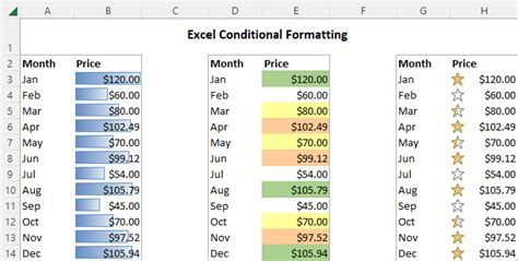
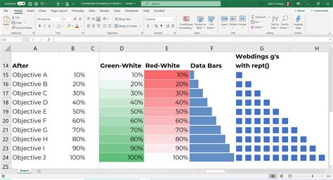
Visualizing Data: By using different colors for different text values, you can create a quick visual representation of your data.

Advanced Conditional Formatting Techniques

For more complex scenarios, you can combine multiple conditions using the AND or OR functions within your formulas. For example, to highlight cells that contain both "example" and "test," you could use a formula like =AND(ISNUMBER(SEARCH("example",A1)),ISNUMBER(SEARCH("test",A1))).

Troubleshooting Common Issues

Rules Not Applying: Make sure the formula is correct and the formatting options are set as desired.
Incorrect Cells Highlighted: Check that the rule is applied to the correct range of cells.
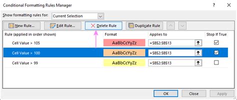
Rules Conflicting: If you have multiple rules, they might conflict. Try rearranging the order of the rules or using the "Stop If True" option.

Gallery of Conditional Formatting Examples

Conditional Formatting Image Gallery

Advanced Formulas for Conditional Formatting

Data Visualization with Conditional Formatting

Troubleshooting Tips for Conditional Formatting

Best Practices for Using Conditional Formatting

Tutorials for Mastering Conditional Formatting

FAQs

What is Conditional Formatting in Excel?

Conditional Formatting is a feature in Excel that allows you to format cells based on the values of those cells. It enables you to highlight cells that meet specific conditions, making it easier to visualize and analyze data.

How do I apply Conditional Formatting to change cell color based on text?

To apply Conditional Formatting, select the cells, go to the Home tab, click on Conditional Formatting, choose "New Rule," and then select "Use a formula to determine which cells to format." Enter a formula that checks for the text you're interested in, and then click "Format" to choose the formatting options.

Can I use Conditional Formatting with formulas that check multiple conditions?

Yes, you can use the AND and OR functions within your formulas to check multiple conditions. This allows for more complex and specific formatting rules.

How do I troubleshoot issues with Conditional Formatting not applying correctly?

Check that the formula is correct, the formatting options are set as desired, and the rule is applied to the correct range of cells. Also, ensure that there are no conflicting rules.

Are there any best practices for using Conditional Formatting effectively?

Yes, keep your rules simple and well-organized, use clear and descriptive formulas, and limit the number of rules applied to a range to avoid conflicts and improve performance.

In conclusion, changing Excel cell color based on text is a powerful feature that can significantly enhance your spreadsheet's readability and usability. By mastering Conditional Formatting and understanding how to apply it effectively, you can create more informative, visually appealing, and easy-to-understand Excel worksheets. Whether you're working with simple text searches or complex conditions, Excel's Conditional Formatting feature has the tools you need to make your data stand out. Feel free to share your experiences or ask questions about using Conditional Formatting in the comments below, and don't forget to share this article with anyone who might benefit from learning more about this versatile Excel feature.