Intro
Learn how to color rows in Excel using formulas, conditional formatting, and VBA macros, making data analysis and visualization easier with row highlighting and shading techniques.
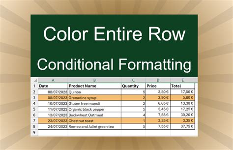
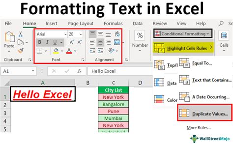
Coloring rows in Excel can greatly enhance the readability and visual appeal of your spreadsheets. It can help in distinguishing between different types of data, highlighting important information, and making your data more engaging. Whether you're working on a personal budget, a business report, or any other type of spreadsheet, learning how to color rows in Excel is a valuable skill. In this article, we'll delve into the various methods of coloring rows in Excel, exploring both manual and automated techniques.
The importance of coloring rows in Excel cannot be overstated. It's not just about aesthetics; it's also about functionality. By using different colors for different rows, you can quickly identify patterns, trends, and anomalies in your data. This can be particularly useful in large datasets where it might be challenging to analyze data without some form of visual differentiation. Moreover, coloring rows can make your spreadsheet more user-friendly, especially when sharing it with others who may not be as familiar with the data as you are.
Before we dive into the specifics of how to color rows in Excel, it's worth noting that Excel offers a wide range of tools and features that can help you customize your spreadsheet. From basic formatting options to more advanced conditional formatting rules, Excel provides everything you need to make your data stand out. Whether you're a beginner or an advanced user, understanding how to utilize these features can significantly improve your productivity and the overall quality of your work.
Manual Row Coloring

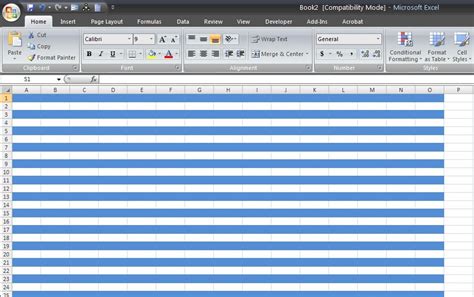
Manual row coloring is the simplest way to add color to your rows in Excel. This method involves selecting the rows you want to color and then applying the desired color using the formatting options available in the Excel ribbon. To manually color rows, follow these steps:
- Select the rows you want to color by clicking on the row headers. You can select multiple rows by holding down the Ctrl key while clicking on each row header.
- Go to the "Home" tab in the Excel ribbon.
- Click on the "Fill Color" button in the "Font" group. This button looks like a paint bucket.
- Choose the color you want to apply to your rows from the color palette.
Benefits of Manual Row Coloring
Manual row coloring offers several benefits, including the ability to quickly and easily add color to specific rows without needing to create rules or formulas. It's ideal for small datasets or for situations where you need to make one-time changes to your spreadsheet. However, for larger datasets or for situations where you need to apply consistent formatting based on specific conditions, manual coloring might not be the most efficient approach.Conditional Row Coloring
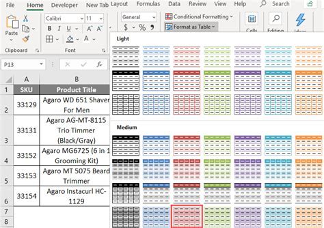
Conditional row coloring, on the other hand, allows you to automatically apply colors to rows based on specific conditions or rules. This feature is incredibly powerful and can help you highlight important information, identify trends, and more. To use conditional row coloring, follow these steps:
- Select the range of cells you want to format.
- Go to the "Home" tab in the Excel ribbon.
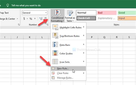
- Click on the "Conditional Formatting" button in the "Styles" group.
- Choose "New Rule" to create a new formatting rule.
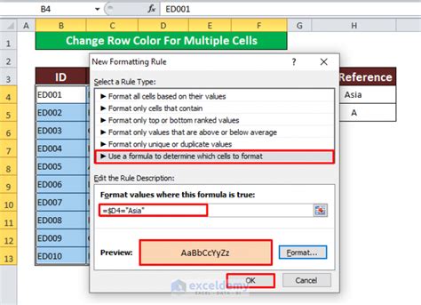
- Select the type of rule you want to create, such as "Format values where this formula is true."
- Enter your formula or select the formatting options you want to apply.
- Click "OK" to apply the rule.
Types of Conditional Formatting Rules
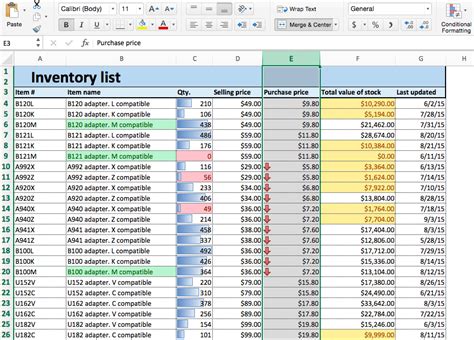
Excel offers several types of conditional formatting rules, including: - Highlight Cells Rules: These rules allow you to highlight cells based on specific conditions, such as values greater than or less than a certain number, or cells that contain specific text. - Top/Bottom Rules: These rules enable you to highlight the top or bottom percentage of values in a range, or the top or bottom n items in a range. - Data Bars: These rules display data bars in cells to represent the value in each cell relative to other cells in the range. - Color Scales: These rules apply a color scale to a range of cells to represent the relative values of the cells.Using Formulas for Row Coloring

Using formulas for row coloring provides another level of flexibility and automation. By leveraging Excel's formula capabilities, you can create complex rules that apply colors based on a wide range of conditions. To use formulas for row coloring, you typically need to combine the formula with the conditional formatting feature. For example, you might use a formula to identify cells that meet a certain condition and then apply a specific color to those cells.
Example Formulas for Row Coloring
Here are a few examples of formulas you might use for row coloring: - `=A1>10` to highlight cells in column A that are greater than 10. - `=ISBLANK(A1)` to highlight blank cells in column A. - `=TODAY()-A1>30` to highlight dates in column A that are more than 30 days old.Best Practices for Row Coloring

When it comes to row coloring in Excel, there are several best practices to keep in mind. First, it's essential to use colors consistently throughout your spreadsheet to avoid confusion. Second, choose colors that provide sufficient contrast with the background and other elements in your spreadsheet. Third, avoid overusing colors, as this can make your spreadsheet look cluttered and difficult to read. Finally, consider using themes or built-in formatting options to ensure that your row coloring aligns with the overall design of your spreadsheet.
Common Mistakes to Avoid
Some common mistakes to avoid when coloring rows in Excel include: - Inconsistent color usage: Failing to use colors consistently can make your spreadsheet look disorganized and may confuse users. - Insufficient contrast: Using colors that are too similar to the background or other elements can make your spreadsheet difficult to read. - Overuse of colors: Applying too many different colors can clutter your spreadsheet and detract from its usability.Excel Row Coloring Image Gallery


How do I color rows in Excel based on a condition?
+To color rows in Excel based on a condition, use the conditional formatting feature. Select the range of cells, go to the "Home" tab, click on "Conditional Formatting," and then choose "New Rule" to create a rule based on your condition.
Can I use formulas to color rows in Excel?
+Yes, you can use formulas to color rows in Excel. Combine your formula with the conditional formatting feature to apply colors based on specific conditions.
What are the best practices for row coloring in Excel?
+Best practices for row coloring in Excel include using colors consistently, choosing colors that provide sufficient contrast, avoiding the overuse of colors, and considering the use of themes or built-in formatting options.
In conclusion, coloring rows in Excel is a versatile and powerful feature that can significantly enhance the usability and visual appeal of your spreadsheets. Whether you're using manual coloring, conditional formatting, or formulas, Excel provides the tools you need to make your data stand out. By following the best practices outlined in this article and exploring the various techniques and resources available, you can unlock the full potential of row coloring in Excel and take your spreadsheet skills to the next level. We invite you to share your experiences, tips, and questions about row coloring in Excel in the comments below, and don't forget to share this article with anyone who might benefit from learning more about this valuable skill.