Highlight Minimum Value In Excel Rows

Highlighting the minimum value in Excel rows can be a useful feature for quickly identifying the smallest value in a dataset. This can be particularly helpful for analyzing data, such as finding the lowest score, the smallest value in a list of prices, or the minimum value in a series of measurements. Excel provides several ways to achieve this, including using conditional formatting, formulas, and pivot tables. In this article, we will explore the different methods to highlight the minimum value in Excel rows, making it easier for you to work with your data.

Introduction to Conditional Formatting

Conditional formatting is a powerful tool in Excel that allows you to highlight cells based on specific conditions, such as values, formulas, or formatting. To highlight the minimum value in a row using conditional formatting, you can follow these steps:

Select the range of cells that you want to format.
Go to the "Home" tab in the Excel ribbon.
Click on "Conditional Formatting" in the "Styles" group.
Select "New Rule."
Choose "Use a formula to determine which cells to format."
Enter the formula =MIN($A1:$E1)=A1, assuming your data is in row 1 from column A to E. Adjust the formula according to your data range.
Click "Format" and choose how you want to highlight the cells (e.g., fill color, font color).
Click "OK" to apply the rule.

Using Formulas to Identify Minimum Values

Another approach to highlighting the minimum value in a row is by using formulas. You can use the MIN function in Excel to find the smallest value in a range of cells. Here’s how you can do it:

Assume your data is in cells A1 to E1.
In a new cell, say F1, enter the formula =MIN(A1:E1).
This will give you the minimum value in the range A1:E1.
To highlight the cell containing the minimum value, you can use conditional formatting based on the formula, as described in the previous section.

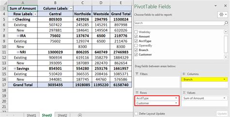
Pivot Tables for Data Analysis

Pivot tables are a great tool for summarizing and analyzing large datasets. While they might not directly highlight the minimum value in a row, they can be used to find and display minimum values across different categories or rows.

Select your data range.
Go to the "Insert" tab and click on "PivotTable."
Choose a cell to place the pivot table and click "OK."
In the "PivotTable Fields" pane, drag the field you want to analyze to the "Values" area.
Right-click on the field in the "Values" area and select "Value Field Settings."
Under "Summarize by," choose "Min" to display the minimum value.

Steps to Highlight Minimum Value

To make the process clearer, here are the steps to highlight the minimum value in a row using conditional formatting:

Select Your Data: Choose the range of cells you want to analyze.
Apply Conditional Formatting: Use the formula =MIN($A1:$E1)=A1 (adjusting for your data range) to highlight the minimum value.
Format Your Cells: Select a format to highlight the minimum value, such as a fill color.
Apply to Other Rows: If you have multiple rows, you can apply the same rule to each row or use a single rule that applies to all rows by adjusting the formula accordingly.

Benefits of Highlighting Minimum Values

Highlighting the minimum value in Excel rows offers several benefits, including:

Quick Identification: It allows for the quick identification of the smallest value in a dataset.
Data Analysis: It aids in data analysis by visually distinguishing the minimum value from other data points.
Decision Making: By easily identifying minimum values, users can make informed decisions based on their data.

Common Challenges and Solutions

When highlighting the minimum value, you might encounter challenges such as:

Multiple Minimum Values: If there are multiple cells with the same minimum value, all of them will be highlighted.
Non-Numeric Data: The MIN function and conditional formatting based on it will not work correctly if your range includes non-numeric data.
Dynamic Ranges: If your data range changes frequently, you might need to adjust your formulas and conditional formatting rules accordingly.

Gallery of Excel Formatting

Excel Formatting Gallery

Frequently Asked Questions

How do I highlight the minimum value in Excel using conditional formatting?

To highlight the minimum value, select your data range, go to the "Home" tab, click on "Conditional Formatting," select "New Rule," and use a formula like `=MIN($A1:$E1)=A1` to format the cells.

Can I use formulas to find and highlight the minimum value in a row?

Yes, you can use the MIN function in a formula to find the minimum value. For example, `=MIN(A1:E1)` will give you the minimum value in the range A1:E1. You can then use conditional formatting based on this formula to highlight the cell.

How do I apply the same conditional formatting rule to multiple rows in Excel?

To apply the same rule to multiple rows, you can either apply the rule individually to each row or adjust your formula to apply to all rows at once. For example, using `=MIN($A1:$E1)=A1` and then dragging the format down to other rows will apply the rule to each row based on its own minimum value.

In conclusion, highlighting the minimum value in Excel rows is a straightforward process that can significantly aid in data analysis and decision-making. By using conditional formatting, formulas, or pivot tables, you can easily identify and highlight the smallest value in your dataset. Remember to adjust your approach based on the specifics of your data and the tools available in Excel. If you have any further questions or need more detailed guidance on any of the steps outlined, don’t hesitate to ask. Share your experiences or tips on working with Excel in the comments below, and consider sharing this article with others who might find it useful.