Show Parentheses For Negative Numbers In Excel

When working with financial data or any numerical information in Excel, it's often helpful to visually distinguish between positive and negative numbers. One common way to do this is by showing parentheses around negative numbers, which can make your spreadsheets more readable and easier to understand at a glance. In this article, we'll explore how to show parentheses for negative numbers in Excel, along with some additional formatting tips to enhance your spreadsheet's clarity and usability.

The importance of clear and consistent formatting in Excel cannot be overstated. It not only makes your spreadsheets look more professional but also aids in the quick identification of trends, errors, or areas that require attention. Formatting negative numbers with parentheses is a simple yet effective way to achieve this clarity. Whether you're working on a personal budget, a business financial report, or any other type of numerical data analysis, learning how to apply this formatting will be beneficial.

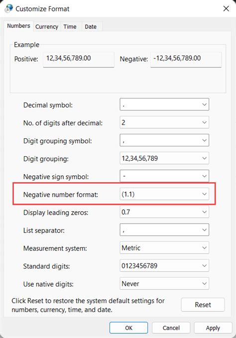
To get started with showing parentheses for negative numbers, you first need to understand how Excel handles number formatting. Excel provides a wide range of formatting options that can be applied to cells, including how numbers are displayed. For negative numbers, the default setting might simply display them with a minus sign (-), but you can easily change this to enclose them in parentheses instead. This customization not only applies to negative numbers but can also be tailored to positive numbers, zeros, and even text within the same cell, allowing for a high degree of flexibility in how your data is presented.

How to Show Parentheses for Negative Numbers

Show Parentheses for Negative Numbers in Excel

To format cells so that negative numbers are displayed with parentheses in Excel, follow these steps:

Select the Cells: Choose the cells that you want to apply the formatting to. This could be a single cell, a range of cells, or an entire column.
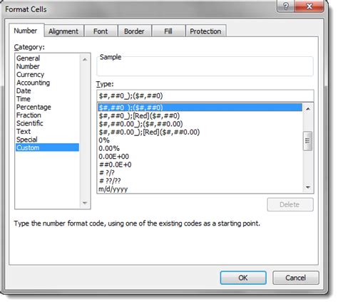
Open the Format Cells Dialog: Right-click on the selected cells and choose "Format Cells" from the context menu. Alternatively, you can use the keyboard shortcut Ctrl + 1 (Windows) or Command + 1 (Mac) to quickly open the Format Cells dialog.
Select the Number Tab: In the Format Cells dialog, click on the "Number" tab.
Choose the Category: Under the Category list, select "Custom". This option allows you to define a custom format for your numbers.
Enter the Custom Format: In the "Type" field, you will see a box where you can enter your custom format. To display negative numbers with parentheses, you need to enter a format code. For example, to format numbers with two decimal places and show negative numbers in parentheses, you would enter: #,##0.00_);(#,##0.00). The #,##0.00 part formats positive numbers, and the (#,##0.00) part formats negative numbers by enclosing them in parentheses.
Apply the Format: Click "OK" to apply the custom format to your selected cells.

Understanding Custom Number Formats

Custom number formats in Excel are powerful tools that allow you to control exactly how your numbers are displayed. The format code is divided into sections separated by semicolons (;), each section defining the format for a specific type of value: positive numbers, negative numbers, zeros, and text.

The first section (before the first semicolon) defines the format for positive numbers.
The second section (between the first and second semicolons) defines the format for negative numbers.
The third section (after the second semicolon) defines the format for zeros.
The fourth section (after the third semicolon) defines the format for text.

For example, the format code #,##0.00_);(#,##0.00);("Zero");(@) would:

Format positive numbers with two decimal places (e.g., 1234.56).
Format negative numbers with two decimal places enclosed in parentheses (e.g., (1234.56)).
Display the text "Zero" for zero values.
Display text as is.

Additional Formatting Tips

Beyond formatting negative numbers with parentheses, Excel offers a plethora of other formatting options to enhance the readability and usability of your spreadsheets. Here are a few additional tips:

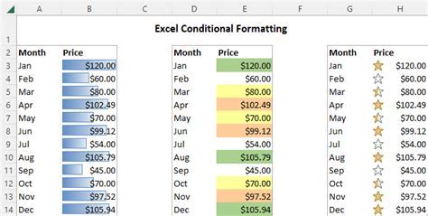
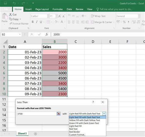
Conditional Formatting: Use conditional formatting to highlight cells based on specific conditions, such as values above or below a certain threshold, or to identify duplicate values.
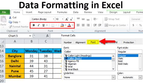
Number Formatting: Experiment with different number formats to find the one that best suits your data. This could include formats for percentages, currencies, dates, and times.
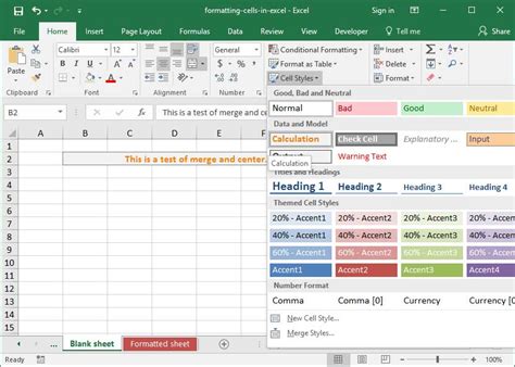
Font and Color: Adjust the font, font size, and color to make your spreadsheet more visually appealing and to draw attention to important information.
Alignment: Properly align your data within cells to improve readability. This could include left-aligning text, right-aligning numbers, or using center alignment for headings.

Gallery of Excel Formatting Examples

Excel Formatting Gallery

Frequently Asked Questions

How do I format negative numbers in Excel to show parentheses?

To format negative numbers to show parentheses in Excel, select the cells you want to format, open the Format Cells dialog, go to the Number tab, select Custom, and then enter a custom format code such as #,##0.00_);(#,##0.00).

What is the purpose of custom number formats in Excel?

Custom number formats in Excel allow you to control how numbers are displayed, enabling you to format positive numbers, negative numbers, zeros, and text differently within the same cell.

How can I apply conditional formatting in Excel?

To apply conditional formatting, select the cells you want to format, go to the Home tab, find the Styles group, click on Conditional Formatting, and then choose the type of formatting you want to apply, such as Highlight Cells Rules or Top/Bottom Rules.

In conclusion, showing parentheses for negative numbers in Excel is a straightforward process that can significantly enhance the clarity and readability of your spreadsheets. By mastering custom number formats and exploring the various formatting options available in Excel, you can create professional-looking spreadsheets that effectively communicate your data insights. Whether you're a beginner or an advanced Excel user, taking the time to learn and apply these formatting techniques will undoubtedly improve your workflow and the overall quality of your work. We invite you to share your own tips and experiences with Excel formatting in the comments below, and don't forget to share this article with anyone who might benefit from learning more about how to make their spreadsheets stand out.