Index And Match In Google Sheets

The ability to index and match data in Google Sheets is a powerful tool for data analysis and manipulation. Indexing and matching functions allow users to look up and retrieve data from a table or range based on specific criteria, making it easier to manage and analyze large datasets. In this article, we will delve into the world of indexing and matching in Google Sheets, exploring the various functions and techniques used to achieve these tasks.

Indexing and matching are essential skills for anyone working with data in Google Sheets, as they enable users to extract specific information from a dataset and perform complex data analysis tasks. By mastering these functions, users can streamline their workflow, reduce errors, and gain valuable insights from their data. Whether you are a student, a business professional, or a data enthusiast, understanding how to index and match data in Google Sheets is crucial for unlocking the full potential of this powerful spreadsheet software.

The importance of indexing and matching in Google Sheets cannot be overstated. These functions are used in a wide range of applications, from simple data lookups to complex data analysis and visualization tasks. By learning how to use indexing and matching functions, users can create dynamic and interactive spreadsheets that update automatically when new data is added or changed. This makes it easier to track changes, identify trends, and make informed decisions based on data-driven insights.

Introduction To Index And Match Functions

The INDEX and MATCH functions are two of the most powerful and versatile functions in Google Sheets. The INDEX function returns a value at a specified position in a range or array, while the MATCH function returns the relative position of a value within a range or array. When used together, these functions enable users to look up and retrieve data from a table or range based on specific criteria.

The INDEX function has the following syntax: INDEX(range, row, column). The range is the range of cells that contains the data, the row is the row number of the value to be returned, and the column is the column number of the value to be returned. The MATCH function has the following syntax: MATCH(lookup_value, lookup_array, [match_type]). The lookup_value is the value to be looked up, the lookup_array is the range of cells that contains the data, and the match_type is the type of match to be performed.

Using The Index Function

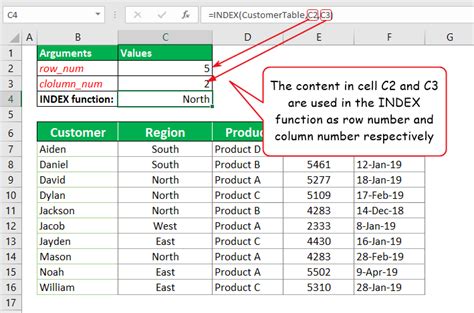
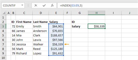
The INDEX function is used to return a value at a specified position in a range or array. For example, suppose we have a range of cells A1:B2 that contains the following data: A1: John B1: 25 A2: Jane B2: 30 To return the value in cell B1, we can use the following formula: INDEX(A1:B2, 1, 2). This formula returns the value 25, which is the value in cell B1.

Using The Match Function

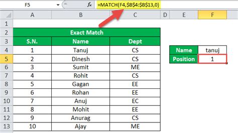
The MATCH function is used to return the relative position of a value within a range or array. For example, suppose we have a range of cells A1:A2 that contains the following data: A1: John A2: Jane To return the position of the value "Jane", we can use the following formula: MATCH("Jane", A1:A2, 0). This formula returns the value 2, which is the position of the value "Jane" in the range A1:A2.

Combining Index And Match Functions

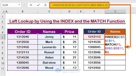
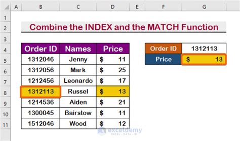
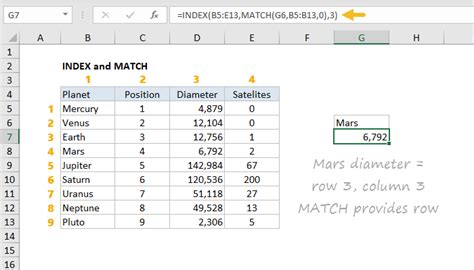
The INDEX and MATCH functions can be combined to create a powerful lookup formula. The INDEX function is used to return a value at a specified position in a range or array, while the MATCH function is used to return the relative position of a value within a range or array. By combining these functions, users can look up and retrieve data from a table or range based on specific criteria.

For example, suppose we have a table of data that contains the following information: A1: Name B1: Age A2: John B2: 25 A3: Jane B3: 30 To return the age of a person with the name "Jane", we can use the following formula: INDEX(B2:B3, MATCH("Jane", A2:A3, 0)). This formula returns the value 30, which is the age of the person with the name "Jane".

Using Index And Match With Multiple Criteria

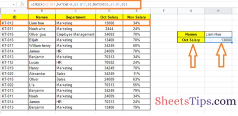
The INDEX and MATCH functions can also be used with multiple criteria. For example, suppose we have a table of data that contains the following information: A1: Name B1: Age C1: City A2: John B2: 25 C2: New York A3: Jane B3: 30 C3: Los Angeles To return the age of a person with the name "Jane" and the city "Los Angeles", we can use the following formula: INDEX(B2:B3, MATCH(1, (A2:A3="Jane") * (C2:C3="Los Angeles"), 0)). This formula returns the value 30, which is the age of the person with the name "Jane" and the city "Los Angeles".

Real-World Applications Of Index And Match Functions

The INDEX and MATCH functions have a wide range of real-world applications. These functions can be used to create dynamic and interactive spreadsheets that update automatically when new data is added or changed. They can also be used to perform complex data analysis tasks, such as data filtering, data grouping, and data visualization.

For example, suppose we have a spreadsheet that contains sales data for a company. The spreadsheet has the following columns: A1: Date B1: Product C1: Sales To return the total sales for a specific product, we can use the following formula: SUMIFS(C2:C100, B2:B100, "Product A"). This formula returns the total sales for the product "Product A".

However, if we want to return the total sales for a specific product and date, we can use the following formula: INDEX(C2:C100, MATCH(1, (B2:B100="Product A") * (A2:A100="2022-01-01"), 0)). This formula returns the total sales for the product "Product A" on the date "2022-01-01".

Using Index And Match With Other Google Sheets Functions

The INDEX and MATCH functions can also be used with other Google Sheets functions, such as the SUMIFS, AVERAGEIFS, and COUNTIFS functions. For example, suppose we have a spreadsheet that contains sales data for a company. The spreadsheet has the following columns: A1: Date B1: Product C1: Sales To return the total sales for a specific product and date, we can use the following formula: SUMIFS(C2:C100, B2:B100, "Product A", A2:A100, "2022-01-01"). This formula returns the total sales for the product "Product A" on the date "2022-01-01".

However, if we want to return the average sales for a specific product and date, we can use the following formula: AVERAGEIFS(C2:C100, B2:B100, "Product A", A2:A100, "2022-01-01"). This formula returns the average sales for the product "Product A" on the date "2022-01-01".

Best Practices For Using Index And Match Functions

When using the INDEX and MATCH functions, there are several best practices to keep in mind. First, make sure to use absolute references when referencing ranges or arrays. This will ensure that the formula returns the correct value, even if the range or array is moved or changed.

Second, use the MATCH function to return the relative position of a value within a range or array, rather than hard-coding the position. This will make the formula more flexible and easier to maintain.

Third, use the INDEX function to return a value at a specified position in a range or array, rather than using the OFFSET function. This will make the formula more efficient and easier to understand.

Finally, test the formula thoroughly to ensure that it returns the correct value. This can be done by checking the formula against a sample dataset, or by using the formula to perform a complex data analysis task.

Common Errors When Using Index And Match Functions

When using the INDEX and MATCH functions, there are several common errors to watch out for. First, make sure to use the correct syntax for the formula. This includes using the correct number of arguments, and using the correct data types for each argument.

Second, make sure to use absolute references when referencing ranges or arrays. This will ensure that the formula returns the correct value, even if the range or array is moved or changed.

Third, make sure to test the formula thoroughly to ensure that it returns the correct value. This can be done by checking the formula against a sample dataset, or by using the formula to perform a complex data analysis task.

Finally, be careful when using the INDEX and MATCH functions with other Google Sheets functions, such as the SUMIFS, AVERAGEIFS, and COUNTIFS functions. This can cause errors or unexpected results, especially if the functions are not used correctly.

Index And Match Functions Image Gallery

What is the INDEX function in Google Sheets?

+

The INDEX function returns a value at a specified position in a range or array.

What is the MATCH function in Google Sheets?

+

The MATCH function returns the relative position of a value within a range or array.

How do I use the INDEX and MATCH functions together?

+

The INDEX and MATCH functions can be used together to look up and retrieve data from a table or range based on specific criteria.

What are some common errors to watch out for when using the INDEX and MATCH functions?

+

Some common errors to watch out for include using the wrong syntax, not using absolute references, and not testing the formula thoroughly.

How can I use the INDEX and MATCH functions with other Google Sheets functions?

+

The INDEX and MATCH functions can be used with other Google Sheets functions, such as the SUMIFS, AVERAGEIFS, and COUNTIFS functions, to perform complex data analysis tasks.

In conclusion, the INDEX and MATCH functions are powerful tools for data analysis and manipulation in Google Sheets. By understanding how to use these functions, users can create dynamic and interactive spreadsheets that update automatically when new data is added or changed. Whether you are a student, a business professional, or a data enthusiast, mastering the INDEX and MATCH functions is essential for unlocking the full potential of Google Sheets. We encourage you to try out these functions and explore their many applications in data analysis and visualization. Share your experiences and tips with us in the comments below, and don't forget to share this article with others who may benefit from learning about the INDEX and MATCH functions in Google Sheets.