5 Ways Vlookup

The Vlookup function is one of the most powerful and versatile tools in Excel, allowing users to search for and retrieve data from a table based on a specific value. This function has numerous applications in data analysis, reporting, and management, making it an essential skill for anyone working with spreadsheets. In this article, we will explore five ways to use the Vlookup function, including its basic syntax, advanced applications, and troubleshooting tips.

The Vlookup function is often used to retrieve data from a large dataset, such as a customer database or an inventory list. By using Vlookup, users can quickly and easily find specific information, such as a customer's address or the price of a product. The function is also useful for data validation, allowing users to ensure that data is accurate and consistent across the spreadsheet.

One of the key benefits of the Vlookup function is its ability to simplify complex data analysis tasks. By using Vlookup, users can quickly and easily retrieve data from a large dataset, without having to manually search through the data. This can save a significant amount of time and reduce the risk of errors, making it an essential tool for anyone working with large datasets.

What is Vlookup?

The Vlookup function is a built-in Excel function that allows users to search for a value in a table and return a corresponding value from another column. The function has four arguments: the value to search for, the table to search in, the column to return a value from, and an optional range lookup argument. The basic syntax of the Vlookup function is: VLOOKUP(lookup_value, table_array, col_index_num, [range_lookup]).

How to Use Vlookup

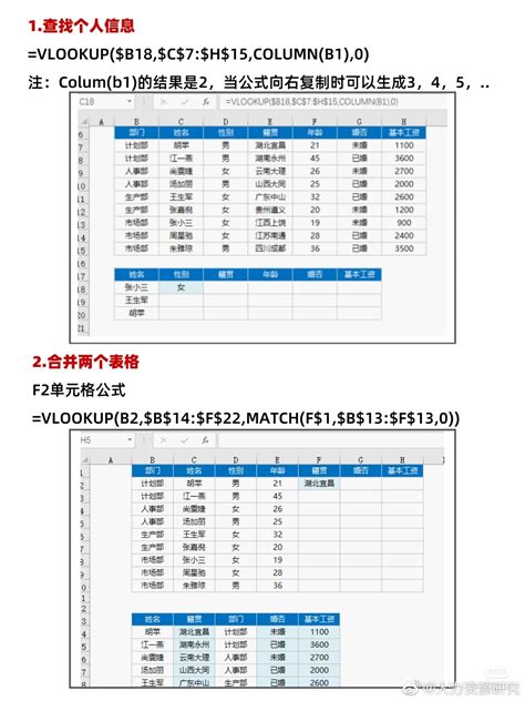
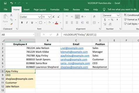
To use the Vlookup function, users must first select the cell where they want to display the result. Then, they must enter the Vlookup formula, specifying the value to search for, the table to search in, and the column to return a value from. The function will then search for the specified value in the table and return the corresponding value from the specified column.

5 Ways to Use Vlookup

Here are five ways to use the Vlookup function: * Retrieving data from a table: The most basic use of the Vlookup function is to retrieve data from a table based on a specific value. For example, if you have a table of customer information, you can use Vlookup to retrieve a customer's address based on their name or ID number. * Data validation: The Vlookup function can be used to validate data in a spreadsheet. For example, if you have a list of product codes, you can use Vlookup to check if a specific code is valid and retrieve the corresponding product name. * Creating drop-down lists: The Vlookup function can be used to create drop-down lists in Excel. For example, if you have a list of countries, you can use Vlookup to create a drop-down list of cities based on the selected country. * Retrieving data from multiple tables: The Vlookup function can be used to retrieve data from multiple tables. For example, if you have two tables, one with customer information and another with order information, you can use Vlookup to retrieve the customer's name and order total based on the order ID. * Performing calculations: The Vlookup function can be used to perform calculations based on data in a table. For example, if you have a table of prices and discounts, you can use Vlookup to calculate the discounted price of a product based on the original price and discount percentage.

Vlookup Syntax and Arguments

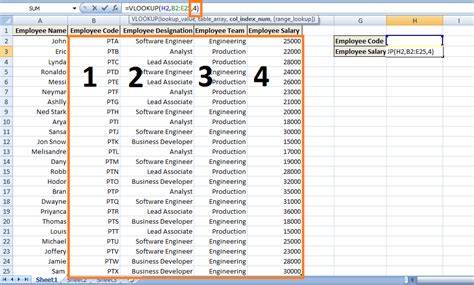
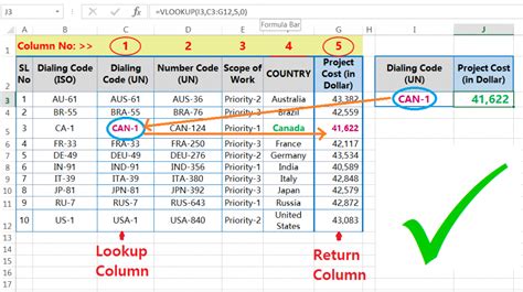
The Vlookup function has four arguments: the value to search for, the table to search in, the column to return a value from, and an optional range lookup argument. The basic syntax of the Vlookup function is: VLOOKUP(lookup_value, table_array, col_index_num, [range_lookup]).

Lookup_value: The value to search for in the table.
Table_array: The table to search in.
Col_index_num: The column to return a value from.
Range_lookup: An optional argument that specifies whether to perform an exact or approximate match.

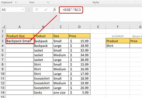
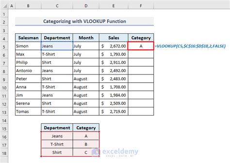
Vlookup Examples

Here are some examples of using the Vlookup function: * Retrieving a customer's address based on their name: =VLOOKUP(A2, customer_table, 2, FALSE) * Retrieving a product's price based on its code: =VLOOKUP(A2, product_table, 3, FALSE) * Creating a drop-down list of cities based on the selected country: =VLOOKUP(A2, country_table, 2, FALSE)

Vlookup Errors and Troubleshooting

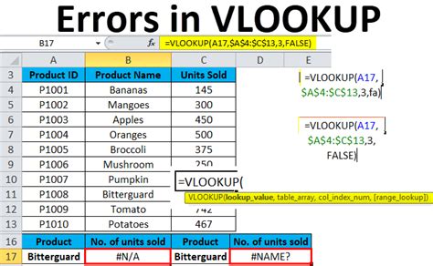
The Vlookup function can return several types of errors, including: * #N/A: The value was not found in the table. * #REF!: The column index is greater than the number of columns in the table. * #VALUE!: The lookup value is not a number or text string.

To troubleshoot Vlookup errors, users can check the following:

Make sure the lookup value is spelled correctly and matches the format of the values in the table.
Make sure the column index is correct and within the range of columns in the table.
Make sure the table array is correctly specified and includes the column to return a value from.

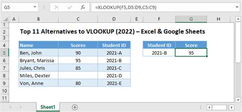
Vlookup Alternatives

There are several alternatives to the Vlookup function, including: * INDEX/MATCH: This function combination is more flexible and powerful than Vlookup and can be used to retrieve data from multiple tables. * LOOKUP: This function is similar to Vlookup but can be used to retrieve data from a range of cells instead of a table. * FILTER: This function can be used to retrieve data from a table based on multiple criteria.

Vlookup Best Practices

Here are some best practices to keep in mind when using the Vlookup function: * Use absolute references for the table array and column index to avoid errors when copying the formula. * Use the FALSE argument for range_lookup to perform an exact match. * Use the Vlookup function with other functions, such as INDEX/MATCH, to create more complex and powerful formulas.

Vlookup Image Gallery

What is the Vlookup function in Excel?

The Vlookup function is a built-in Excel function that allows users to search for a value in a table and return a corresponding value from another column.

How do I use the Vlookup function?

To use the Vlookup function, select the cell where you want to display the result, enter the Vlookup formula, and specify the value to search for, the table to search in, and the column to return a value from.

What are some common errors when using the Vlookup function?

Common errors when using the Vlookup function include #N/A, #REF!, and #VALUE! errors, which can be caused by incorrect lookup values, column indexes, or table arrays.

What are some alternatives to the Vlookup function?

Alternatives to the Vlookup function include the INDEX/MATCH function combination, the LOOKUP function, and the FILTER function.

What are some best practices for using the Vlookup function?

Best practices for using the Vlookup function include using absolute references, performing exact matches, and using the function with other functions to create more complex and powerful formulas.

We hope this article has provided you with a comprehensive understanding of the Vlookup function and its applications in Excel. Whether you are a beginner or an advanced user, mastering the Vlookup function can help you to work more efficiently and effectively with data in Excel. If you have any further questions or would like to share your own experiences with the Vlookup function, please don't hesitate to comment below. Additionally, if you found this article helpful, please share it with others who may benefit from learning about the Vlookup function.