Intro
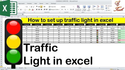
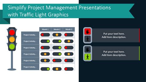
Create a dynamic traffic light system in Excel sheets using formulas and conditional formatting, enhancing data visualization with red, yellow, and green indicators for instant status updates and decision-making.
The concept of a traffic light system in an Excel sheet is a powerful tool for data analysis and visualization. It allows users to quickly and easily identify trends, patterns, and outliers in their data, making it an essential component of many business and financial applications. In this article, we will delve into the world of traffic light systems in Excel, exploring their importance, benefits, and implementation.
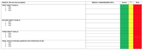
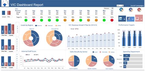
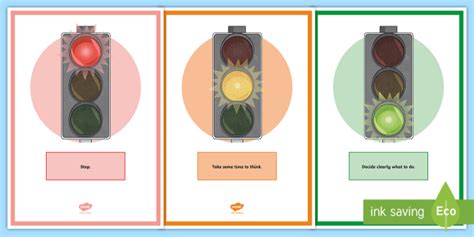
The traffic light system is a simple yet effective way to visualize data in Excel. It uses three colors - red, yellow, and green - to indicate different states or conditions, such as good, average, or poor performance. This system is widely used in various fields, including finance, marketing, and operations, to help users make informed decisions and take corrective actions. By using a traffic light system, users can quickly identify areas that require attention, making it an indispensable tool for data-driven decision-making.
The importance of traffic light systems in Excel cannot be overstated. They provide a clear and concise way to communicate complex data insights, enabling users to focus on the most critical aspects of their business. By using a traffic light system, users can identify trends and patterns in their data, anticipate potential problems, and make data-driven decisions to drive business growth. Moreover, traffic light systems are highly customizable, allowing users to tailor them to their specific needs and requirements.
Implementing Traffic Light Systems in Excel

Implementing a traffic light system in Excel is relatively straightforward. Users can use conditional formatting to create a traffic light system, which involves setting up rules to format cells based on their values. For example, users can set up a rule to format cells with values above a certain threshold as green, cells with values below a certain threshold as red, and cells with values within a certain range as yellow. This can be done using the conditional formatting feature in Excel, which allows users to create custom formatting rules based on formulas and values.
Steps to Create a Traffic Light System in Excel
To create a traffic light system in Excel, follow these steps: * Select the cells that you want to format using the traffic light system. * Go to the Home tab in the Excel ribbon and click on the Conditional Formatting button. * Select New Rule from the dropdown menu. * Choose the type of rule that you want to create, such as "Format values where this formula is true". * Enter the formula that you want to use to determine the formatting, such as `=A1>10` to format cells with values above 10 as green. * Click on the Format button to select the formatting that you want to apply, such as a green fill color. * Repeat the process to create rules for yellow and red formatting.Benefits of Traffic Light Systems in Excel

The benefits of traffic light systems in Excel are numerous. They provide a clear and concise way to visualize data, enabling users to quickly identify trends and patterns. Traffic light systems also help users to focus on the most critical aspects of their business, allowing them to prioritize their efforts and resources. Additionally, traffic light systems are highly customizable, enabling users to tailor them to their specific needs and requirements.
Some of the key benefits of traffic light systems in Excel include:
- Improved data visualization: Traffic light systems provide a clear and concise way to visualize data, enabling users to quickly identify trends and patterns.
- Enhanced decision-making: By using a traffic light system, users can make informed decisions and take corrective actions to drive business growth.
- Increased productivity: Traffic light systems help users to focus on the most critical aspects of their business, allowing them to prioritize their efforts and resources.
- Customizability: Traffic light systems are highly customizable, enabling users to tailor them to their specific needs and requirements.
Best Practices for Using Traffic Light Systems in Excel
To get the most out of traffic light systems in Excel, follow these best practices: * Use a consistent color scheme: Use a consistent color scheme throughout your Excel sheet to avoid confusion and ensure that users can quickly understand the meaning of each color. * Keep it simple: Avoid using too many colors or complex formatting rules, as this can make it difficult for users to understand the traffic light system. * Use clear and concise labels: Use clear and concise labels to explain the meaning of each color and the rules that are used to determine the formatting. * Test and refine: Test your traffic light system and refine it as necessary to ensure that it is working correctly and providing the desired insights.Common Applications of Traffic Light Systems in Excel

Traffic light systems are widely used in various fields, including finance, marketing, and operations. Some common applications of traffic light systems in Excel include:
- Financial analysis: Traffic light systems can be used to analyze financial data, such as revenue, expenses, and profits, to identify trends and patterns.
- Marketing analysis: Traffic light systems can be used to analyze marketing data, such as website traffic, social media engagement, and customer acquisition costs, to identify areas for improvement.
- Operational analysis: Traffic light systems can be used to analyze operational data, such as production levels, inventory levels, and supply chain performance, to identify areas for improvement.
Real-World Examples of Traffic Light Systems in Excel
Here are some real-world examples of traffic light systems in Excel: * A financial analyst uses a traffic light system to analyze revenue data, with green indicating revenue above $10,000, yellow indicating revenue between $5,000 and $10,000, and red indicating revenue below $5,000. * A marketing manager uses a traffic light system to analyze website traffic data, with green indicating traffic above 1,000 visitors per day, yellow indicating traffic between 500 and 1,000 visitors per day, and red indicating traffic below 500 visitors per day. * An operations manager uses a traffic light system to analyze production data, with green indicating production levels above 90%, yellow indicating production levels between 80% and 90%, and red indicating production levels below 80%.Traffic Light Systems Image Gallery
What is a traffic light system in Excel?
+A traffic light system in Excel is a way to visualize data using three colors - red, yellow, and green - to indicate different states or conditions.
How do I create a traffic light system in Excel?
+To create a traffic light system in Excel, use the conditional formatting feature to set up rules to format cells based on their values.
What are the benefits of using a traffic light system in Excel?
+The benefits of using a traffic light system in Excel include improved data visualization, enhanced decision-making, increased productivity, and customizability.
In conclusion, traffic light systems in Excel are a powerful tool for data analysis and visualization. By using a traffic light system, users can quickly and easily identify trends and patterns in their data, make informed decisions, and take corrective actions to drive business growth. Whether you are a financial analyst, marketing manager, or operations manager, a traffic light system in Excel can help you to achieve your goals and improve your overall performance. So why not give it a try and see the benefits for yourself? Share your experiences and insights with us, and don't forget to comment below with your thoughts on traffic light systems in Excel.