Vlookup Google Sheets From Another Workbook

The VLOOKUP function is a powerful tool in Google Sheets that allows users to search for and retrieve data from a table based on a specific value. While it's commonly used within the same workbook, it can also be used to retrieve data from another workbook. In this article, we'll explore how to use VLOOKUP in Google Sheets to retrieve data from another workbook, and provide tips and examples to help you get the most out of this function.

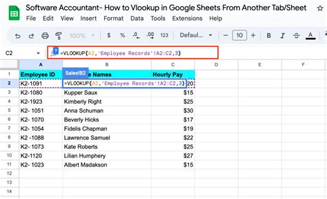
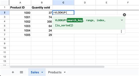
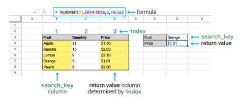
To start, let's take a look at the basic syntax of the VLOOKUP function: VLOOKUP(search_key, range, index, [is_sorted]). The search_key is the value you want to search for, range is the table or range of cells that contains the data you want to retrieve, index is the column number that contains the value you want to return, and [is_sorted] is an optional argument that specifies whether the data is sorted.

When using VLOOKUP to retrieve data from another workbook, you'll need to use the IMPORTRANGE function to import the data from the other workbook. The IMPORTRANGE function allows you to import a range of cells from another Google Sheets workbook. The syntax for IMPORTRANGE is: IMPORTRANGE(spreadsheet_url, range_string). The spreadsheet_url is the URL of the workbook you want to import data from, and range_string is the range of cells you want to import.

Here's an example of how you might use VLOOKUP and IMPORTRANGE together:

Let's say you have two workbooks: "Workbook A" and "Workbook B". Workbook A contains a table with the following data: | Name | Age | City | | --- | --- | --- | | John | 25 | New York | | Jane | 30 | Los Angeles | | Bob | 35 | Chicago | You want to use VLOOKUP in Workbook B to retrieve the age of John from Workbook A. First, you would use the `IMPORTRANGE` function to import the data from Workbook A: `=IMPORTRANGE("https://docs.google.com/spreadsheets/d/WorkbookA_ID", "Sheet1!A1:C3")` This imports the data from the range A1:C3 in Sheet1 of Workbook A.

Next, you would use the VLOOKUP function to retrieve the age of John: =VLOOKUP("John", IMPORTRANGE("https://docs.google.com/spreadsheets/d/WorkbookA_ID", "Sheet1!A1:C3"), 2, FALSE) This searches for the value "John" in the first column of the imported data, and returns the value in the second column (the age).

Benefits of Using VLOOKUP with IMPORTRANGE

Using VLOOKUP with `IMPORTRANGE` allows you to retrieve data from another workbook without having to copy and paste the data. This can be especially useful when working with large datasets or when you need to retrieve data from a workbook that is updated frequently.

Some benefits of using VLOOKUP with `IMPORTRANGE` include: * Reduced errors: By importing data directly from another workbook, you can reduce the risk of errors caused by manual data entry. * Increased efficiency: Using VLOOKUP with `IMPORTRANGE` can save you time and effort by automating the process of retrieving data from another workbook. * Improved collaboration: By using VLOOKUP with `IMPORTRANGE`, you can collaborate with others on a workbook without having to share the entire workbook.

Step-by-Step Guide to Using VLOOKUP with IMPORTRANGE

Here's a step-by-step guide to using VLOOKUP with `IMPORTRANGE`: 1. Open the workbook you want to retrieve data from (Workbook A). 2. Note the URL of Workbook A. 3. Open the workbook you want to use to retrieve the data (Workbook B). 4. Use the `IMPORTRANGE` function to import the data from Workbook A: `=IMPORTRANGE("https://docs.google.com/spreadsheets/d/WorkbookA_ID", "Sheet1!A1:C3")` 5. Use the VLOOKUP function to retrieve the data: `=VLOOKUP("John", IMPORTRANGE("https://docs.google.com/spreadsheets/d/WorkbookA_ID", "Sheet1!A1:C3"), 2, FALSE)` 6. Press Enter to execute the formula.

Note: You may need to authorize the import of data from Workbook A by clicking on the "Allow access" button.

Troubleshooting Common Issues with VLOOKUP and IMPORTRANGE

Here are some common issues you may encounter when using VLOOKUP with `IMPORTRANGE`, along with some troubleshooting tips: * Error message: "Cannot connect to external spreadsheet" + Solution: Check that the URL of the external spreadsheet is correct, and that the spreadsheet is publicly accessible. * Error message: "Invalid range" + Solution: Check that the range specified in the `IMPORTRANGE` function is correct, and that it matches the range of cells you want to import. * Error message: "VLOOKUP cannot find the value" + Solution: Check that the value you are searching for exists in the first column of the imported data, and that the data is sorted correctly.

By following these troubleshooting tips, you can resolve common issues and get the most out of using VLOOKUP with `IMPORTRANGE`.

Best Practices for Using VLOOKUP with IMPORTRANGE

Here are some best practices to keep in mind when using VLOOKUP with `IMPORTRANGE`: * Use the correct syntax: Make sure to use the correct syntax for both the `IMPORTRANGE` and VLOOKUP functions. * Specify the correct range: Make sure to specify the correct range of cells to import and search. * Use absolute references: Use absolute references (e.g. `$A$1`) instead of relative references (e.g. `A1`) to ensure that the formula works correctly. * Test the formula: Test the formula to ensure it is working correctly before using it in your workbook.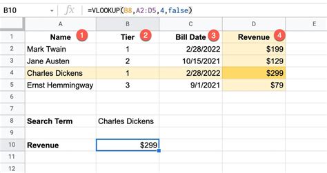

By following these best practices, you can ensure that your VLOOKUP formula works correctly and efficiently.

Conclusion and Next Steps

In this article, we've explored how to use VLOOKUP in Google Sheets to retrieve data from another workbook. We've covered the benefits of using VLOOKUP with `IMPORTRANGE`, provided a step-by-step guide to using the formula, and offered troubleshooting tips and best practices.

To take your skills to the next level, try practicing with different examples and scenarios. You can also explore other Google Sheets functions, such as INDEX/MATCH or QUERY, to see which one works best for your needs.

Vlookup Google Sheets Image Gallery

What is VLOOKUP in Google Sheets?

+

VLOOKUP is a function in Google Sheets that allows you to search for and retrieve data from a table based on a specific value.

How do I use VLOOKUP with IMPORTRANGE?

+

To use VLOOKUP with IMPORTRANGE, you need to use the IMPORTRANGE function to import the data from another workbook, and then use the VLOOKUP function to retrieve the data.

What are the benefits of using VLOOKUP with IMPORTRANGE?

+

The benefits of using VLOOKUP with IMPORTRANGE include reduced errors, increased efficiency, and improved collaboration.

We hope this article has been helpful in explaining how to use VLOOKUP in Google Sheets to retrieve data from another workbook. If you have any questions or need further assistance, please don't hesitate to ask. Share this article with your friends and colleagues who may find it useful, and let us know in the comments below if you have any other questions or topics you'd like us to cover.