Intro
Learn to Vlookup two columns in Excel using formulas and functions, including index-match, lookup tables, and multiple criteria to retrieve data efficiently.
Vlookup is a powerful function in Excel that allows users to search for a value in a table and return a corresponding value from another column. While the traditional Vlookup function is used to search for a value in one column and return a value from another column, there are times when you need to Vlookup two columns in Excel. This can be useful when you need to search for a combination of values in two columns and return a corresponding value from another column.
In this article, we will explore the different ways to Vlookup two columns in Excel, including using the Vlookup function with multiple criteria, using the Index-Match function, and using the Filter function. We will also provide examples and step-by-step instructions to help you master these techniques.
Understanding Vlookup Function

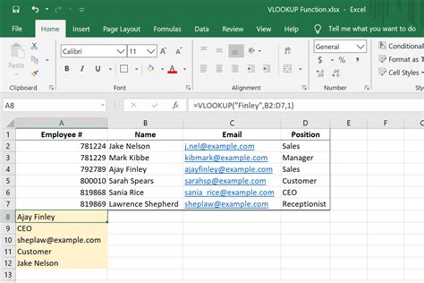
The Vlookup function is a built-in function in Excel that allows you to search for a value in a table and return a corresponding value from another column. The syntax for the Vlookup function is VLOOKUP(lookup_value, table_array, col_index_num, [range_lookup]). The lookup_value is the value you want to search for, table_array is the range of cells that contains the data, col_index_num is the column number that contains the value you want to return, and [range_lookup] is an optional argument that specifies whether you want to search for an exact match or an approximate match.
Vlookup Two Columns Using Vlookup Function

To Vlookup two columns using the Vlookup function, you can use the & operator to concatenate the two columns. For example, if you want to search for a combination of values in columns A and B, you can use the formula =VLOOKUP(A2&B2, table_array, col_index_num, [range_lookup]). This formula concatenates the values in cells A2 and B2 and searches for the resulting value in the table_array.
Here's an example:
| Employee ID | Department | Name |
|---|---|---|
| 101 | Sales | John Smith |
| 102 | Marketing | Jane Doe |
| 103 | Sales | Bob Johnson |
If you want to search for an employee with ID 101 and department Sales, you can use the formula =VLOOKUP(101&"Sales", A:B, 3, FALSE). This formula concatenates the values 101 and "Sales" and searches for the resulting value in the range A:B. The col_index_num argument is set to 3, which means the formula returns the value in the third column (Name).
Using Index-Match Function
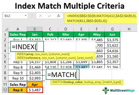
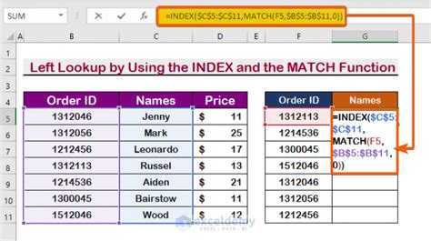
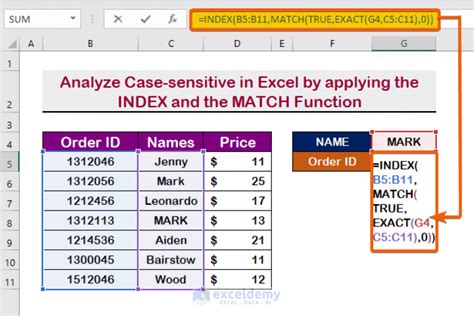
Another way to Vlookup two columns in Excel is to use the Index-Match function. The Index-Match function is a more flexible and powerful function than the Vlookup function, and it allows you to search for a value in multiple columns.
The syntax for the Index-Match function is INDEX(range, MATCH(lookup_value, lookup_array, [match_type]). The range is the range of cells that contains the data, lookup_value is the value you want to search for, lookup_array is the range of cells that contains the values you want to search, and [match_type] is an optional argument that specifies whether you want to search for an exact match or an approximate match.
To Vlookup two columns using the Index-Match function, you can use the formula =INDEX(range, MATCH(1, (A:A=101)*(B:B="Sales"), 0)). This formula searches for the value 101 in column A and the value "Sales" in column B, and returns the corresponding value in the range range.
Using Filter Function
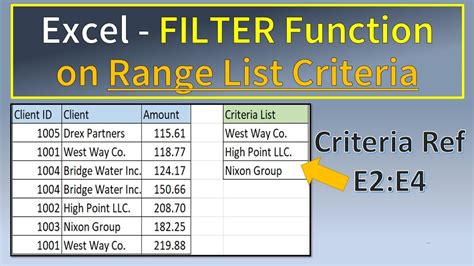
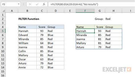
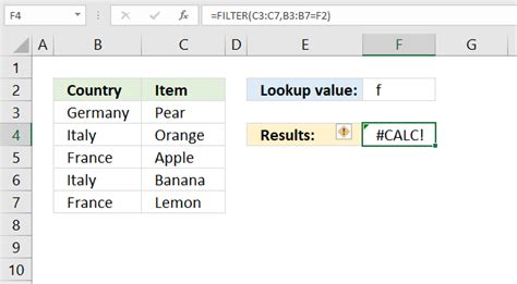
The Filter function is a new function in Excel that allows you to filter a range of cells based on multiple criteria. To Vlookup two columns using the Filter function, you can use the formula =FILTER(range, (A:A=101)*(B:B="Sales")). This formula filters the range range based on the criteria A:A=101 and B:B="Sales", and returns the corresponding values.
Benefits of Using Filter Function
The Filter function has several benefits over the Vlookup function and the Index-Match function. It is more flexible and allows you to filter a range of cells based on multiple criteria. It also returns multiple values, whereas the Vlookup function and the Index-Match function return only one value.Common Errors When Using Vlookup Function
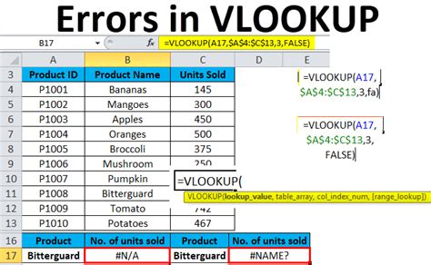
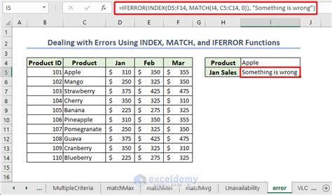
When using the Vlookup function, there are several common errors that you need to avoid. One of the most common errors is the `#N/A` error, which occurs when the Vlookup function cannot find the value you are searching for. To avoid this error, you need to make sure that the value you are searching for exists in the range `table_array`.Another common error is the #REF error, which occurs when the column index col_index_num is greater than the number of columns in the range table_array. To avoid this error, you need to make sure that the column index col_index_num is correct.
Vlookup Function Image Gallery


What is the Vlookup function in Excel?
+The Vlookup function is a built-in function in Excel that allows you to search for a value in a table and return a corresponding value from another column.
How do I use the Vlookup function to search for a value in two columns?
+To use the Vlookup function to search for a value in two columns, you can use the `&` operator to concatenate the two columns. For example, if you want to search for a combination of values in columns A and B, you can use the formula `=VLOOKUP(A2&B2, table_array, col_index_num, [range_lookup])`.
What is the Index-Match function in Excel?
+The Index-Match function is a more flexible and powerful function than the Vlookup function, and it allows you to search for a value in multiple columns.
How do I use the Filter function to Vlookup two columns in Excel?
+To use the Filter function to Vlookup two columns in Excel, you can use the formula `=FILTER(range, (A:A=101)*(B:B="Sales"))`. This formula filters the range `range` based on the criteria `A:A=101` and `B:B="Sales"`, and returns the corresponding values.
What are the benefits of using the Filter function over the Vlookup function and the Index-Match function?
+The Filter function has several benefits over the Vlookup function and the Index-Match function. It is more flexible and allows you to filter a range of cells based on multiple criteria. It also returns multiple values, whereas the Vlookup function and the Index-Match function return only one value.
In summary, Vlookup two columns in Excel can be done using the Vlookup function, the Index-Match function, or the Filter function. Each function has its own benefits and drawbacks, and the choice of which function to use depends on the specific needs of your project. By mastering these functions, you can become more proficient in using Excel and improve your productivity. We hope this article has been helpful in explaining the different ways to Vlookup two columns in Excel. If you have any further questions or need more information, please don't hesitate to ask. Share this article with your friends and colleagues who may benefit from learning about Vlookup two columns in Excel.