Intro
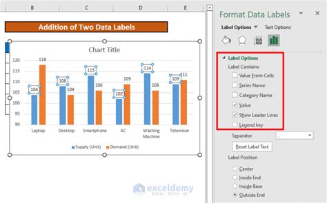
Enhance Excel charts by adding two data labels, improving visualization and readability with custom labels, data points, and chart formatting techniques.
Adding data labels to an Excel chart can greatly enhance its readability and provide viewers with a quick understanding of the data points. Data labels are text or numeric values that are displayed directly on the chart, next to or above/below each data point, making it easier to see the exact values without having to hover over the points or refer to the data table. Here's a step-by-step guide on how to add two data labels to an Excel chart, along with explanations and examples to help you understand the process better.
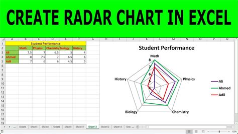
When you're working with charts in Excel, one of the most effective ways to make your data more understandable is by using data labels. These labels can display the value of each data point, the series name, the category name, or even custom text. For instance, if you have a column chart showing sales figures for different regions, adding data labels can help viewers quickly identify the sales amount for each region without having to look at the axis.
To get started with adding data labels to your Excel chart, first ensure that your chart is selected. You can do this by clicking on the chart area. Once your chart is selected, you'll see the "Chart Design" and "Chart Format" tabs appear in the ribbon. These tabs provide various tools for customizing your chart's appearance and functionality.
Step 1: Selecting the Chart
Click on the chart you want to add data labels to. This action will activate the chart tools in the ribbon, specifically the "Chart Design" and "Chart Format" tabs.
Step 2: Adding Data Labels
- Go to the "Chart Design" tab.
- Click on the "Add Chart Element" button in the "Chart Layouts" group.
- From the dropdown menu, select "Data Labels".
- Choose where you want the data labels to be positioned, such as "Center" for a pie chart or "Inside End" for a column or bar chart.
Alternatively, if you want more control over the data labels, such as adding labels from another range or specifying a new data range:
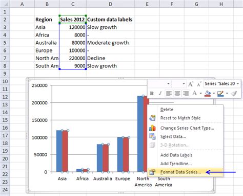
- Right-click on the data series in your chart (e.g., a column in a column chart).
- Select "Format Data Point" or "Format Data Series".
- In the task pane that opens, go to the "Series Options" or "Data Labels" section, depending on your Excel version.
- Check the box next to "Data Labels" and then click on "Data Label Options" or "Data Labels" to customize the label's appearance and content.
Step 3: Customizing Data Labels
After adding data labels, you might want to customize them to better suit your needs. Here's how you can do it:
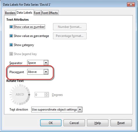
- Right-click on one of the data labels and select "Format Data Labels".
- In the task pane, you can choose what you want to display in the data label, such as "Value", "Value from Cells", "Category Name", "Series Name", etc.
- For more advanced customization, such as changing the label's position, format, or adding a separator, explore the other options available in the task pane.
Step 4: Adding a Second Data Label
If you want to add another type of data label (for example, adding both the value and the percentage for each data point in a pie chart), you can do so by:
- Right-clicking on the data series again.
- Selecting "Format Data Point" or "Format Data Series".
- In the "Data Label Options" section, checking the boxes next to the types of labels you want to display (e.g., "Value" and "Percentage").
Practical Example
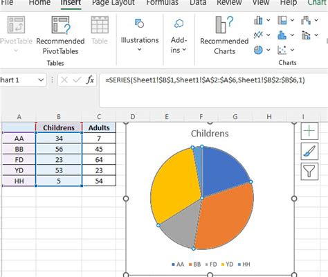
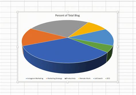
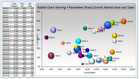
Suppose you have a pie chart showing the market share of different brands. You can add data labels to show both the percentage of market share and the actual sales figure for each brand. To do this:
- First, add the data labels as described above.
- Then, right-click on the pie chart and select "Format Data Series".
- In the task pane, under "Data Labels", check the boxes for both "Percentage" and "Value".
- You can further customize the appearance of these labels, such as changing their position or adding a separator between the percentage and value.
Benefits of Data Labels
Data labels offer several benefits, including:
- Improved Readability: They make it easier for viewers to understand the chart without needing to interpret the axes.
- Precision: Viewers can see the exact values of data points, which is particularly useful in presentations or reports.
- Customization: Excel allows for a high degree of customization, so you can tailor the data labels to fit the needs of your chart and audience.
Tips for Effective Use
- Use Them Sparingly: Too many data labels can clutter the chart. Use them only when necessary for clarity.
- Customize Appearance: Adjust the font, color, and position of data labels to ensure they are readable and do not overlap with other chart elements.
- Consider the Chart Type: Certain chart types, like scatter plots or line charts with many data points, might not benefit from data labels due to potential clutter.
Common Issues
- Overlapping Labels: If your data labels are overlapping, consider rotating them or adjusting their position.
- Inconsistent Formatting: Ensure that all data labels have a consistent format to maintain the chart's professionalism.
Advanced Techniques
For more complex data label needs, such as displaying data from a different range or adding custom text, you might need to delve into Excel's more advanced features, such as using formulas directly within the data label options or leveraging VBA macros for highly customized solutions.
Conclusion and Next Steps
Adding data labels to your Excel charts can significantly enhance their effectiveness in communicating data insights. By following the steps outlined above and experimenting with the various customization options available, you can create charts that are both informative and visually appealing. Remember, the key to using data labels effectively is to strike a balance between providing enough information and avoiding clutter. With practice, you'll become proficient in using data labels to tell compelling stories with your data.

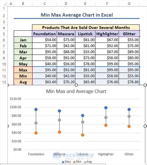
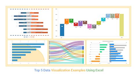

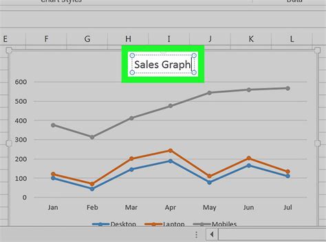
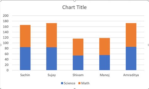
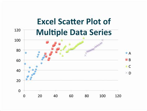
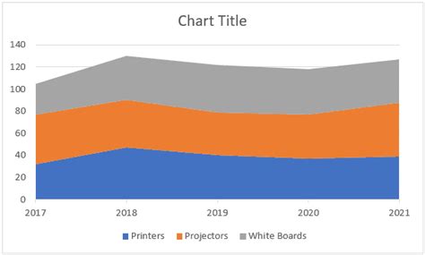
Gallery of Excel Chart Examples
Excel Chart Examples
How do I add data labels to an Excel chart?
+To add data labels, select the chart, go to the "Chart Design" tab, click on "Add Chart Element", and then select "Data Labels". You can also right-click on the data series and select "Format Data Point" or "Format Data Series" to add and customize data labels.
Can I customize the appearance of data labels in Excel?
+Yes, you can customize the appearance of data labels by right-clicking on a data label, selecting "Format Data Label", and then adjusting options such as label position, format, and separator in the task pane.
How do I add a second type of data label to an Excel chart?
+To add a second type of data label, right-click on the data series, select "Format Data Point" or "Format Data Series", go to the "Data Label Options" section, and check the boxes for the types of labels you want to display, such as both "Value" and "Percentage" for a pie chart.
We hope this comprehensive guide has provided you with the knowledge and skills to effectively use data labels in your Excel charts. Whether you're creating simple column charts or complex dashboards, data labels can be a powerful tool in making your data more accessible and understandable. Feel free to share your thoughts or ask questions in the comments below, and don't forget to share this article with others who might benefit from learning about Excel's data labeling capabilities.