Google Sheets Lookup Another Sheet

Looking up data from another sheet in Google Sheets is a fundamental skill that can greatly enhance your spreadsheet management capabilities. Whether you're managing inventory, tracking orders, or analyzing data, the ability to reference and retrieve information from other sheets can streamline your workflow and reduce errors. In this article, we'll delve into the importance of looking up data from another sheet, explore the various methods to achieve this, and provide practical examples to help you master this skill.

The importance of being able to lookup data from another sheet cannot be overstated. It allows for the creation of dynamic and interconnected spreadsheets that can automatically update and reflect changes across different sheets. This is particularly useful in scenarios where data needs to be shared or referenced across multiple sheets, such as in budgeting, where expenses might be listed in one sheet and income in another. By linking these sheets, you can create formulas that automatically calculate totals or balances, making your financial management more accurate and less prone to human error.

Moreover, the ability to lookup data from another sheet is crucial for data analysis. When working with large datasets, it's common to split data into different sheets based on categories or time periods. Being able to reference and compare data across these sheets enables more comprehensive analysis and insights. For instance, in marketing, you might have separate sheets for different campaigns, and looking up data from these sheets can help you compare their performance and make informed decisions about future strategies.

Understanding Google Sheets Lookup Functions

Google Sheets offers several lookup functions that enable you to retrieve data from another sheet. The most commonly used functions include VLOOKUP, INDEX/MATCH, and LOOKUP. Each of these functions has its unique syntax and application, and understanding when to use each can significantly improve your spreadsheet skills.

VLOOKUP: This function looks up a value in the first column of a specified range and returns a value in the same row from another column. The syntax for VLOOKUP is VLOOKUP(lookup_value, table_array, col_index_num, [range_lookup]). It's widely used but can be slow with large datasets and doesn't handle column insertions well.
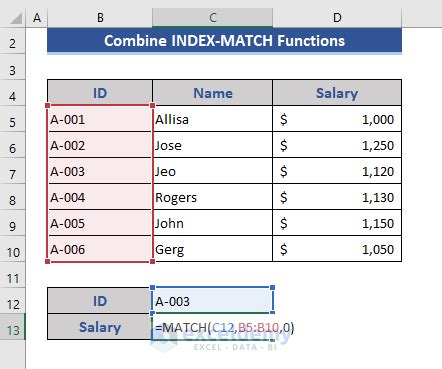
INDEX/MATCH: This combination of functions offers more flexibility and power than VLOOKUP. INDEX returns a value at a specified position in a range, while MATCH looks up a value in a range and returns its position. The syntax for INDEX/MATCH is INDEX(range, MATCH(lookup_value, lookup_array, [match_type]). It's faster and more versatile than VLOOKUP, especially when dealing with large datasets.
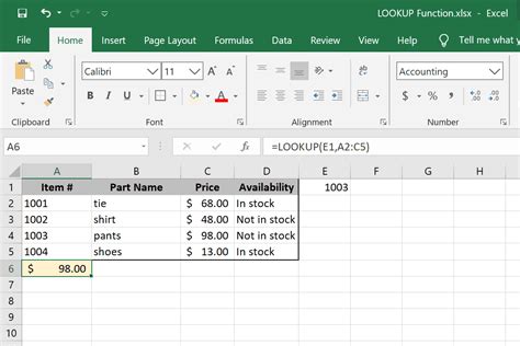
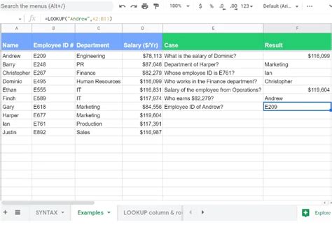
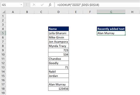
LOOKUP: This function looks up a value in a vector (a row or column) and returns a value from another vector. The syntax for LOOKUP is LOOKUP(lookup_value, lookup_vector, [result_vector]). It's simpler than VLOOKUP and INDEX/MATCH but less flexible.

Step-by-Step Guide to Looking Up Data from Another Sheet

Looking up data from another sheet involves several steps, including preparing your data, choosing the appropriate lookup function, and writing the formula. Here's a step-by-step guide:

Prepare Your Data: Ensure that the data you want to lookup and the data you want to return are in a structured format, typically in tables with headers.
Choose the Lookup Function: Decide which lookup function (VLOOKUP, INDEX/MATCH, or LOOKUP) best suits your needs based on the structure of your data and what you want to achieve.
Write the Formula: Start writing your formula by specifying the lookup value, the range where the lookup value is located, and the column from which you want to return a value.
Reference Another Sheet: To reference another sheet, you need to specify the sheet name followed by an exclamation mark before the range. For example, =VLOOKUP(A2, Sheet2!A:B, 2, FALSE) looks up the value in cell A2 in the first column of the range A:B in Sheet2 and returns the corresponding value in the second column.
Press Enter: After completing your formula, press Enter to execute it. The formula will return the value you're looking for from the other sheet.

Practical Examples

Let's consider a practical example where you have two sheets: "Orders" and "Customers". The "Orders" sheet contains order numbers, customer IDs, and order totals, while the "Customers" sheet contains customer IDs, names, and addresses. You want to lookup the customer name for each order based on the customer ID.

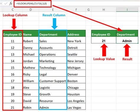
Using VLOOKUP: =VLOOKUP(A2, Customers!A:C, 2, FALSE), where A2 contains the customer ID and Customers!A:C is the range containing customer IDs, names, and addresses.
Using INDEX/MATCH: =INDEX(Customers!B:B, MATCH(A2, Customers!A:A, 0)), where A2 contains the customer ID, Customers!B:B is the range containing customer names, and Customers!A:A is the range containing customer IDs.

Tips and Tricks for Efficient Lookup

Use Absolute References: When referencing another sheet, use absolute references (e.g., $A$2) to ensure that the reference doesn't change when you copy the formula to other cells.
Avoid Using VLOOKUP with Large Datasets: For large datasets, INDEX/MATCH is generally faster and more efficient.
Use Helper Columns: If your lookup is complex, consider using helper columns to break down the lookup process into simpler steps.
Regularly Update Your Data: Ensure that your data is up-to-date and consistent across all sheets to avoid lookup errors.

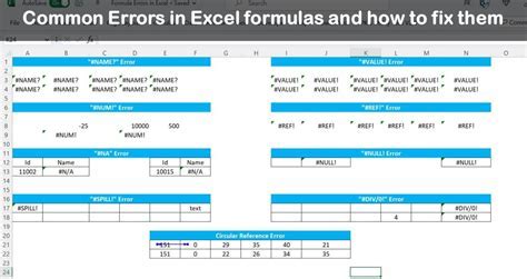
Common Errors and Solutions

#N/A Error: This error occurs when the lookup value is not found. Check for spelling mistakes, ensure the lookup range includes the lookup value, and consider using the IFERROR function to handle such errors.
#REF! Error: This error occurs when the reference to another sheet is incorrect. Check the sheet name and range reference for accuracy.
#VALUE! Error: This error occurs when the formula contains an incorrect value. Check the formula syntax and ensure that all values are correctly referenced.

Google Sheets Lookup Functions Gallery

What is the difference between VLOOKUP and INDEX/MATCH in Google Sheets?

VLOOKUP looks up a value in the first column of a specified range and returns a value in the same row from another column, while INDEX/MATCH offers more flexibility and power, allowing for lookups in any column and returning values from any other column, making it faster and more versatile, especially with large datasets.

How do I reference another sheet in Google Sheets?

To reference another sheet, you specify the sheet name followed by an exclamation mark before the range. For example, `Sheet2!A:B` references the range A:B in Sheet2.

What is the #N/A error in Google Sheets lookup functions, and how do I fix it?

The #N/A error occurs when the lookup value is not found. To fix it, check for spelling mistakes, ensure the lookup range includes the lookup value, and consider using the `IFERROR` function to handle such errors.

In conclusion, looking up data from another sheet in Google Sheets is a powerful feature that can significantly enhance your spreadsheet management and analysis capabilities. By mastering the VLOOKUP, INDEX/MATCH, and LOOKUP functions, you can create dynamic and interconnected spreadsheets that automate tasks and reduce errors. Remember to choose the appropriate function based on your data structure and needs, and don't hesitate to use helper columns or the IFERROR function to handle complex lookups and potential errors. With practice and patience, you'll become proficient in looking up data from another sheet and unlock the full potential of Google Sheets for your data management and analysis needs. We invite you to share your experiences, tips, and tricks for using lookup functions in Google Sheets in the comments below, and don't forget to share this article with anyone who might benefit from mastering these essential skills.