Intro
Changing the cell color based on the value in Excel is a useful feature for highlighting important information, such as high or low values, and making your spreadsheet more visually appealing. This feature is often used in data analysis to quickly identify trends, patterns, or outliers. Excel provides several ways to achieve this, including using Conditional Formatting, which is a powerful tool for formatting cells based on their values.
To get started with changing cell colors based on values, you first need to understand the basics of Conditional Formatting. This feature allows you to apply different formats to cells depending on the value of the cell, the formula that you specify, or based on other conditions. Excel offers several predefined rules that you can use for common formatting tasks, such as highlighting cells that are greater than or less than a specific value, or highlighting cells that contain specific text.
One of the most straightforward ways to change cell color based on value is by using the "Highlight Cells Rules" option within Conditional Formatting. This option provides several predefined rules, including "Greater Than", "Less Than", "Between", "Equal To", and "Text That Contains". For example, if you want to highlight all cells in a range that have a value greater than a certain number, you can use the "Greater Than" rule.
Here's how you can apply Conditional Formatting to change cell color based on value:
- Select the range of cells that you want to format.
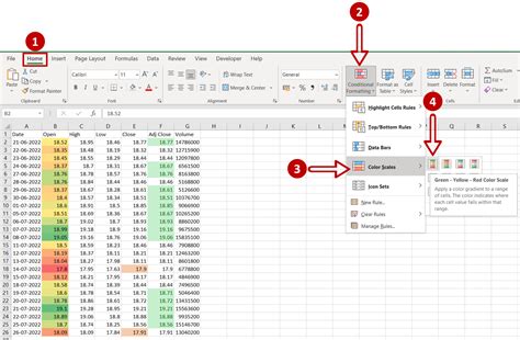
- Go to the "Home" tab on the Excel ribbon.
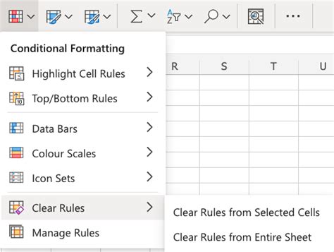
- Click on "Conditional Formatting" in the "Styles" group.
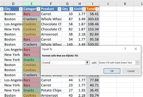
- Choose "Highlight Cells Rules" and then select the appropriate rule based on your needs, such as "Greater Than".
- In the dialog box that appears, enter the value that you want to use as the threshold for formatting.
- Click on the format button to choose the fill color you want to apply to cells that meet the condition.
- Click "OK" to apply the rule.
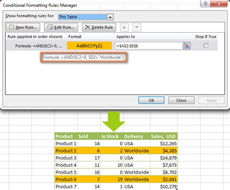
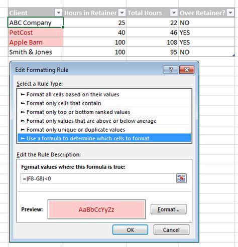
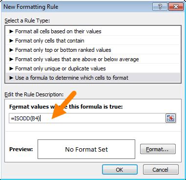
In addition to the predefined rules, you can also use formulas to determine which cells to format. This is particularly useful when you need more complex conditions that are not covered by the predefined rules. To use a formula, you select "New Rule" from the Conditional Formatting dropdown, then choose "Use a formula to determine which cells to format". You can then enter a formula that, if true, will apply the formatting to the cell.
For instance, if you want to highlight cells in column A that contain values greater than the average of the values in column B, you can use a formula like =A1>AVERAGE($B$1:$B$100), assuming your data is in rows 1 through 100. After entering the formula, you click the "Format" button to choose the formatting you want to apply, such as fill color, and then click "OK" to apply the rule.
Advanced Conditional Formatting Techniques
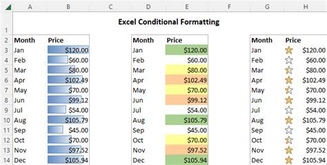
Beyond the basic rules, Conditional Formatting offers more advanced techniques for changing cell colors based on values. One of these techniques involves using multiple conditions. You can apply multiple rules to the same range of cells, allowing you to highlight cells based on different criteria. For example, you could have one rule that highlights cells greater than a certain value in green and another rule that highlights cells less than a different value in red.
Another advanced technique is the use of the "IF" function within your Conditional Formatting formulas. The "IF" function allows you to test a condition and return one value if the condition is true and another value if it is false. This can be particularly useful when you need to apply different formats based on multiple conditions.
Using the "IF" Function in Conditional Formatting
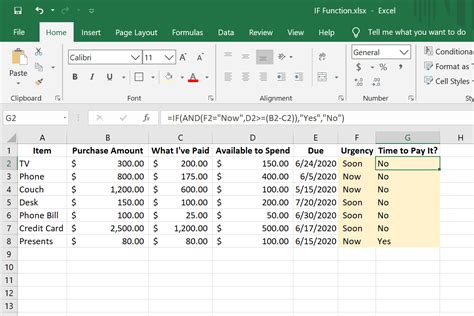
To use the "IF" function in Conditional Formatting, you would follow a similar process to applying a formula-based rule, but your formula would include the "IF" function. For example, if you want to highlight cells in column A that are greater than 10 and less than 20, you could use a formula like =IF(AND(A1>10,A1<20),TRUE,FALSE). This formula checks if the value in cell A1 is between 10 and 20 (exclusive) and returns TRUE if the condition is met and FALSE otherwise.
Managing and Editing Conditional Formatting Rules

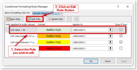
After applying Conditional Formatting rules, you may need to manage or edit them. Excel provides options to view, edit, and delete existing rules. To manage rules, you go back to the Conditional Formatting dropdown, select "Manage Rules", and then you can choose to edit or delete rules as needed. This is useful if your data changes or if you need to adjust the conditions or formats applied to your cells.
Best Practices for Using Conditional Formatting
When using Conditional Formatting to change cell colors based on values, there are several best practices to keep in mind. First, ensure that your rules are clear and well-defined to avoid confusion. It's also a good idea to test your rules on a small set of data before applying them to a larger range. Additionally, consider using named ranges or references to make your formulas more readable and easier to maintain.
In conclusion, changing cell colors based on values in Excel is a powerful feature that can enhance the readability and usefulness of your spreadsheets. By mastering Conditional Formatting and its various options, including the use of formulas and advanced techniques, you can create dynamic and informative spreadsheets that help you and your audience quickly understand complex data.
Conditional Formatting Image Gallery


How do I apply Conditional Formatting to an entire column?
+To apply Conditional Formatting to an entire column, select the column by clicking on the column header, then proceed with the Conditional Formatting steps as you would for a range of cells.
Can I use Conditional Formatting with other Excel features like PivotTables?
+Yes, Conditional Formatting can be used with other Excel features like PivotTables. However, the formatting may not always update dynamically when the PivotTable changes, so you may need to reapply the formatting rules after updating the PivotTable.
How do I copy Conditional Formatting to another range of cells?
+To copy Conditional Formatting to another range of cells, select the cell or range with the formatting, go to the "Home" tab, click on "Format Painter" in the "Clipboard" group, and then select the new range where you want to apply the formatting.
We hope this article has provided you with a comprehensive guide on how to change cell colors based on values in Excel using Conditional Formatting. Whether you're a beginner or an advanced user, mastering this feature can significantly enhance your spreadsheet's usability and visual appeal. If you have any further questions or need more specific guidance, feel free to ask in the comments below. Additionally, if you found this article helpful, please share it with others who might benefit from learning about Conditional Formatting in Excel.