Intro
Learn Excel conditional formatting to compare two columns and highlight cells greater than a value, using formulas, rules, and functions like IF, AND, and OR for dynamic data analysis and visualization.
When working with Excel, conditional formatting is a powerful tool that allows you to highlight cells based on specific conditions, making it easier to analyze and understand your data. One common requirement is to compare two columns and highlight cells where the value in one column is greater than the value in another column. This can be particularly useful for identifying trends, outliers, or specific conditions within your dataset. In this article, we'll explore how to use Excel's conditional formatting feature to compare two columns and highlight cells where the value in one column is greater than the value in another.
To start, let's consider a simple example where we have two columns of data: Column A and Column B. We want to highlight all the cells in Column B where the value is greater than the corresponding value in Column A.

Step 1: Select the Range of Cells
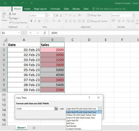
First, select the range of cells in Column B that you want to apply the conditional formatting to. If your data starts from B2 and goes down to B100, you would select the range B2:B100.
Step 2: Open the Conditional Formatting Dialog
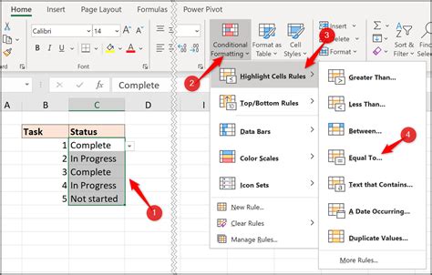
With the range selected, go to the "Home" tab on the Excel ribbon, find the "Styles" group, and click on "Conditional Formatting". This opens a dropdown menu with various options for conditional formatting rules.
Step 3: Create a New Rule
From the dropdown menu, select "New Rule". This opens the "New Formatting Rule" dialog box. Here, you'll choose the type of rule you want to create. Select "Use a formula to determine which cells to format".
Step 4: Enter the Formula
In the formula box, you will enter a formula that compares the values in the two columns. To highlight cells in Column B where the value is greater than the corresponding value in Column A, you would use a formula like =B2>A2. This formula compares the value in cell B2 to the value in cell A2. Since you've selected a range starting from B2, Excel will automatically adjust this formula for each cell in the selected range.
Step 5: Format the Cells
After entering the formula, click on the "Format" button to choose how you want to highlight the cells that meet the condition. You can choose a fill color, font color, border, and more. Once you've selected your formatting options, click "OK".
Step 6: Apply the Rule
Back in the "New Formatting Rule" dialog box, you'll see the formula you entered and a preview of the formatting you chose. Click "OK" to apply the rule. Excel will then highlight all the cells in your selected range where the value is greater than the corresponding value in Column A.
Comparing Columns with Different References
Sometimes, you might need to compare columns where the references are not as straightforward. For example, you might want to compare a cell in Column B with a cell in Column A, but the columns are not adjacent, or you're working with data that spans multiple sheets or workbooks.
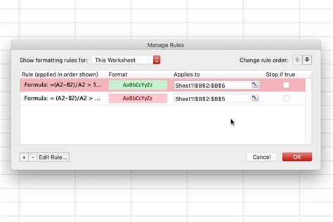
In such cases, you can still use the conditional formatting feature, but you might need to adjust your formula to correctly reference the cells or ranges you're comparing. For instance, if you're comparing cells in Column B with cells in Column D, your formula might look like =B2>D2.
Using Absolute References
If your comparison involves referencing cells or ranges that shouldn't change when the formula is applied across a range of cells, you might need to use absolute references. Absolute references are denoted by a dollar sign ($), such as $A$2 or $D$2. Using absolute references ensures that the formula always references the specified cell or range, regardless of where it's applied.
Tips for Effective Use
- Keep it Simple: Start with simple comparisons and gradually move to more complex formulas as needed.
- Test Your Formula: Before applying conditional formatting, test your formula in a regular cell to ensure it's working as expected.
- Use Relative References Wisely: Relative references (without the dollar sign) are useful for comparing adjacent cells, but be cautious when applying them across large ranges.
Advanced Conditional Formatting Techniques
Beyond simple comparisons, Excel's conditional formatting offers a range of advanced techniques to help you analyze and present your data more effectively. These include:
- Multiple Conditions: You can apply multiple conditions to a range of cells, using the "Add" button in the "New Formatting Rule" dialog box.
- Color Scales: Excel allows you to apply color scales to your data, which can help in visualizing trends or patterns.
- Data Bars: Data bars provide a graphical representation of the data within cells, making it easier to compare values at a glance.
Managing Conditional Formatting Rules
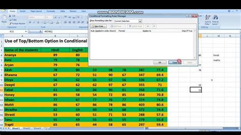
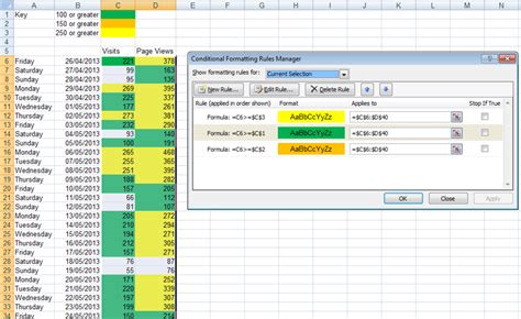
As you apply more conditional formatting rules to your workbook, managing these rules becomes important. Excel provides a "Conditional Formatting Rules Manager" that allows you to view, edit, and delete existing rules. You can access this manager through the "Conditional Formatting" dropdown menu.
Best Practices for Conditional Formatting
- Keep Rules Organized: Use the "Conditional Formatting Rules Manager" to keep your rules organized, especially in complex workbooks.
- Document Your Rules: Consider documenting the rules you've applied, especially if you're working on a shared workbook or if the rules are complex.
Gallery of Conditional Formatting Examples

Conditional Formatting Image Gallery


Frequently Asked Questions
How do I apply conditional formatting to an entire column?
+To apply conditional formatting to an entire column, select the column (e.g., Column B), then follow the steps to create a new rule. Ensure your formula references the first cell of the column (e.g., B2) if you're using a relative reference.
Can I use conditional formatting across multiple sheets or workbooks?
+Yes, you can use conditional formatting across multiple sheets or workbooks by referencing the specific sheet or workbook in your formula. For example, `=B2>Sheet2!A2` compares a cell in the current sheet with a cell in another sheet named "Sheet2".
How do I remove conditional formatting from a range of cells?
+To remove conditional formatting, select the range of cells, go to the "Home" tab, find the "Styles" group, click on "Conditional Formatting", and then select "Clear Rules" > "Clear Rules from Selected Cells".
In conclusion, Excel's conditional formatting feature is a versatile tool that can significantly enhance your data analysis capabilities. By comparing two columns and highlighting cells based on specific conditions, you can gain deeper insights into your data and make more informed decisions. Whether you're working with simple or complex datasets, mastering conditional formatting can help you unlock the full potential of Excel and streamline your workflow. So, explore the various options and techniques available, and discover how conditional formatting can become an indispensable part of your Excel toolkit.