Hide Rows In Google Sheets Based On Value

The ability to hide rows in Google Sheets based on a specific value is a powerful feature that can help you manage and analyze your data more efficiently. This functionality is particularly useful when you have large datasets and need to focus on specific parts of the data without deleting any information. In this article, we will explore how to hide rows in Google Sheets based on a value, the benefits of doing so, and provide step-by-step instructions on how to accomplish this task.

Hiding rows based on values can be achieved through various methods, including using formulas, filters, and Google Apps Script. Each method has its own advantages and is suited for different scenarios. Whether you're a beginner or an advanced user of Google Sheets, understanding how to hide rows based on values can significantly enhance your spreadsheet management skills.

Benefits of Hiding Rows in Google Sheets

Hiding rows in Google Sheets based on specific values offers several benefits. It allows you to:

• Simplify complex datasets by removing unnecessary data from view.
• Focus on specific parts of your data without altering the original dataset.
• Improve data analysis by isolating relevant data points.
• Enhance collaboration by controlling what data team members can see.

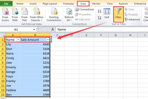
Using Filters to Hide Rows

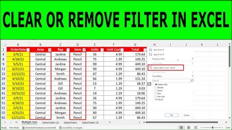
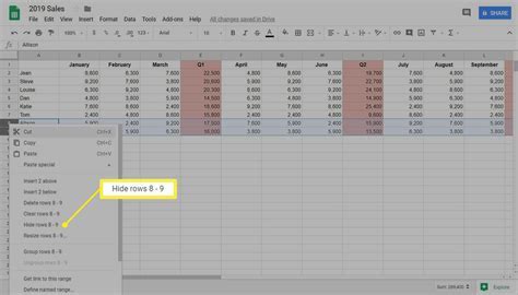
One of the simplest ways to hide rows based on a value is by using filters. Here’s how you can do it:

1. Select the entire range of data you want to filter.
2. Go to the "Data" menu and select "Create a filter".
3. Click on the filter icon that appears in the header of the column you want to filter.
4. Select "Filter by condition" and then choose the condition that matches your needs (e.g., "Text contains", "Greater than", etc.).
5. Enter the value you want to filter by and click "Done".

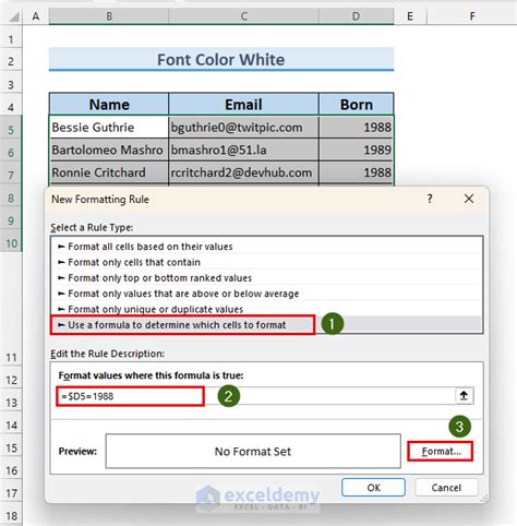
Using Formulas to Hide Rows

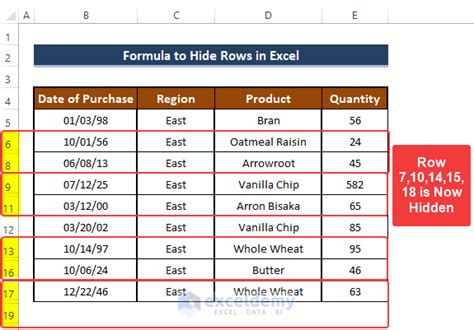
You can also use formulas in combination with conditional formatting to hide rows. Although this method doesn't physically hide rows, it can make them appear hidden by changing their background color to match the sheet's background, effectively making the text invisible.

1. Select the range of cells where you want to apply the formula.
2. Go to the "Format" tab, select "Conditional formatting".
3. In the format cells if dropdown, select "Custom formula is".
4. Enter a formula that returns TRUE if the row should be hidden. For example, =A1="Hide" if you want to hide rows where the value in column A is "Hide".
5. Click "Done" and then apply a background color that matches the sheet's background to "make" the rows appear hidden.

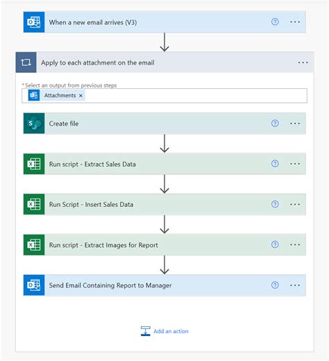
Using Google Apps Script to Hide Rows

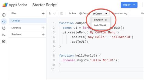
For more advanced and automated solutions, Google Apps Script can be used to hide rows based on values. Here’s a basic example of how to achieve this:

1. Open your Google Sheet.
2. Click on "Tools" > "Script editor" to open the Google Apps Script editor.
3. Delete any code in the editor and paste the following script:

function hideRows() {
  var sheet = SpreadsheetApp.getActiveSpreadsheet().getActiveSheet();
  var dataRange = sheet.getDataRange();
  var values = dataRange.getValues();
  
  for (var i = values.length - 1; i >= 0; i--) {
    if (values[i][0] == "Hide") { // Assuming the value to hide is in the first column
      sheet.hideRows(i + 1);
    }
  }
}

4. Save the script and then run the hideRows function.

Practical Applications

Hiding rows based on values has numerous practical applications across various industries and use cases, such as:

• Data Analysis: Hide rows with missing or irrelevant data to focus on meaningful insights.
• Project Management: Hide completed tasks to focus on ongoing and upcoming tasks.
• Financial Analysis: Hide rows with zero balances or transactions to simplify financial statements.

Gallery of Hiding Rows in Google Sheets

Hiding Rows in Google Sheets Image Gallery

Frequently Asked Questions

How do I hide rows in Google Sheets based on a value?

+

You can hide rows in Google Sheets based on a value by using filters, formulas, or Google Apps Script. The method you choose depends on your specific needs and the complexity of your data.

Can I automate the process of hiding rows in Google Sheets?

+

Yes, you can automate the process of hiding rows in Google Sheets by using Google Apps Script. This allows you to write scripts that can automatically hide rows based on specific conditions.

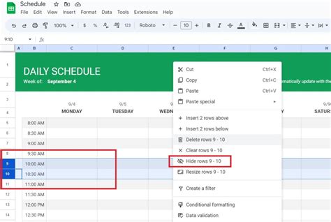
How do I unhide rows in Google Sheets?

+

To unhide rows in Google Sheets, select the rows above and below the hidden row, go to the "Format" menu, select "Hide & unhide", and then click "Unhide rows". Alternatively, you can use the keyboard shortcut Ctrl + Shift + 9 (Windows) or Command + Shift + 9 (Mac).

In conclusion, hiding rows in Google Sheets based on values is a versatile feature that can significantly improve your data management and analysis capabilities. By understanding how to use filters, formulas, and Google Apps Script, you can efficiently manage complex datasets and focus on the data that matters most to your project or analysis. Whether you're working individually or collaborating with a team, mastering the art of hiding rows in Google Sheets can take your productivity to the next level. So, explore these methods, practice using them, and discover how they can enhance your Google Sheets experience. Don't hesitate to share your experiences, ask questions, or provide tips on how you use Google Sheets to manage and analyze your data.