Set Y Intercept To 0 In Excel

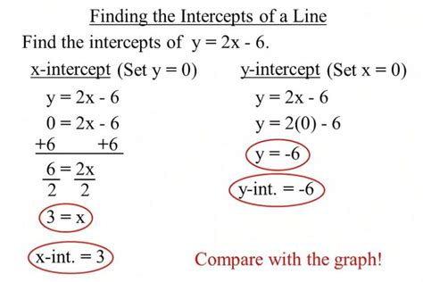
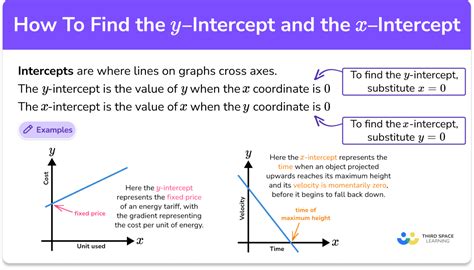
When working with charts and graphs in Excel, it's often necessary to adjust the y-intercept to better visualize and analyze the data. The y-intercept is the point at which the line or curve crosses the y-axis, and setting it to 0 can be particularly useful for certain types of data, such as financial or scientific data, where the zero point has significant meaning. Here's how you can set the y-intercept to 0 in Excel, along with some explanations and examples to guide you through the process.

To begin with, understanding why setting the y-intercept to 0 is important can help you appreciate the value of this adjustment. In many cases, the zero point on the y-axis represents a baseline or a reference point. For instance, in financial analysis, setting the y-intercept to 0 can help in clearly showing profits and losses, as it provides a visual cue for when the values are above or below the zero line.

Now, let's move on to the steps involved in setting the y-intercept to 0 in Excel.

Understanding Excel Charts

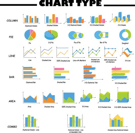
Excel offers a variety of chart types, each suited for different kinds of data and analyses. The process of setting the y-intercept to 0 can vary slightly depending on the type of chart you're using. However, the general steps remain the same across most chart types.

Steps to Set Y Intercept to 0

Select Your Chart: First, you need to select the chart for which you want to adjust the y-intercept. Click on the chart to select it, and you'll see the chart tools appear in the ribbon.
Access Chart Options: With your chart selected, go to the "Chart Tools" in the ribbon. You'll find several tabs here, including "Design," "Layout," and "Format." The exact tab you need might depend on your version of Excel, but generally, you'll find what you need under the "Chart Options" or by right-clicking on the chart.
Adjust Axis Options: Right-click on the y-axis of your chart and select "Format Axis." This will open a sidebar or dialog box where you can adjust various properties of the axis, including where it crosses the x-axis (the y-intercept).
Specify the Intercept: In the axis options, look for the section that allows you to specify the axis crossing point. This might be labeled as "Vertical axis crosses" or something similar. Here, you can choose to set the axis crossing to a specific value, and you want to set this value to 0.
Apply Changes: After setting the y-intercept to 0, apply your changes. Depending on the Excel version, you might need to click "OK" or "Close" to exit the formatting options.

Benefits of Setting Y Intercept to 0

Setting the y-intercept to 0 offers several benefits, including:

Improved Visualization: It can make your chart easier to understand, especially when the zero point has a significant meaning in your data.
Enhanced Analysis: By providing a clear baseline, it can facilitate more accurate analysis and interpretation of the data.
Better Comparisons: When comparing multiple datasets, setting the y-intercept to 0 can help in making direct comparisons by ensuring that all datasets are referenced to the same baseline.

Working with Different Chart Types

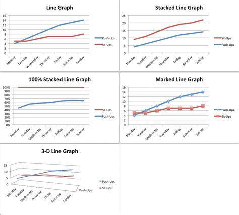
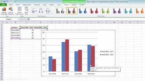
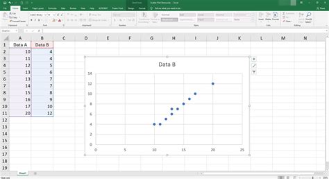
Different chart types in Excel, such as line charts, bar charts, and scatter plots, might have slightly different procedures for setting the y-intercept. However, the core principle remains the same: you're adjusting the axis options to specify where the y-axis crosses the x-axis.

Common Challenges and Solutions

When setting the y-intercept to 0, you might encounter a few challenges, such as the chart not updating as expected or the axis options not being available. Here are some common issues and how to resolve them:

Chart Not Updating: Ensure that you've applied the changes correctly and that the chart is selected when you make the adjustments.
Axis Options Not Available: Check that you're looking at the correct axis (y-axis for setting the y-intercept) and that you've accessed the axis options correctly.

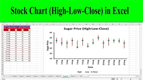
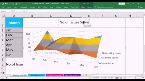
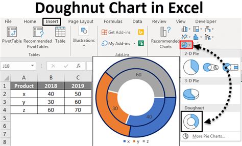
Gallery of Excel Chart Examples

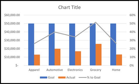
Excel Chart Examples

What is the purpose of setting the y-intercept to 0 in Excel charts?

Setting the y-intercept to 0 in Excel charts is useful for providing a clear baseline for data analysis, especially when the zero point has significant meaning, such as in financial or scientific data.

How do I set the y-intercept to 0 in an Excel chart?

To set the y-intercept to 0, select the chart, access the axis options by right-clicking on the y-axis, and then specify the axis crossing point as 0.

Does setting the y-intercept to 0 work for all types of Excel charts?

The process of setting the y-intercept to 0 is applicable to most chart types in Excel, including line charts, bar charts, and scatter plots, though the exact steps might vary slightly.

In conclusion, setting the y-intercept to 0 in Excel charts is a valuable adjustment that can enhance the clarity and usefulness of your data visualizations. By following the steps outlined above and understanding the benefits and applications of this adjustment, you can improve your data analysis and presentation skills in Excel. Whether you're working with financial data, scientific research, or any other type of data, being able to effectively adjust and customize your charts is crucial for effective communication and analysis. We hope this guide has been helpful in explaining how to set the y-intercept to 0 in Excel and has provided you with the knowledge to create more informative and engaging charts. Feel free to share your thoughts or ask further questions in the comments below.