Excel Formula For Duplicate Check

Checking for duplicates in a dataset is a common task in data analysis, and Excel provides several formulas and functions to accomplish this. The ability to identify duplicate values can help in data cleaning, data validation, and ensuring data integrity. In this article, we will explore various Excel formulas and techniques for checking duplicates, including using the IF function, COUNTIF function, and Conditional Formatting.

The importance of checking for duplicates cannot be overstated. Duplicates can lead to incorrect analysis, skewed results, and poor decision-making. By identifying and managing duplicates, users can ensure their data is accurate, reliable, and consistent. Whether you're working with a small dataset or a large database, Excel's formulas and functions make it easier to detect and handle duplicates.

Excel offers a range of tools and formulas for duplicate checking, from simple to more complex. For beginners, using the IF function combined with the COUNTIF function can provide a straightforward method to identify duplicates. More advanced users might prefer using array formulas or even pivot tables to analyze and summarize their data, including identifying duplicate entries. The choice of method depends on the size of the dataset, the complexity of the data, and the user's familiarity with Excel functions.

Using the IF and COUNTIF Functions

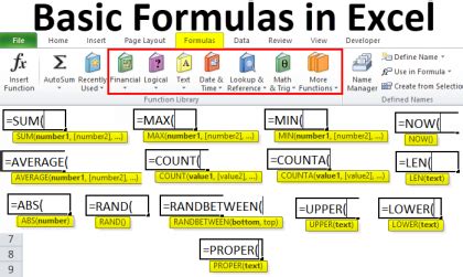
One of the simplest ways to check for duplicates in Excel is by using the IF function in combination with the COUNTIF function. The COUNTIF function counts the number of cells within a range that meet a given condition. By using it to count the occurrences of each value, you can identify duplicates. The formula is as follows:

=IF(COUNTIF(range, cell) > 1, "Duplicate", "Unique")

Here, range is the range of cells you want to check for duplicates, and cell is the cell containing the value you're checking. This formula can be applied to each cell in your dataset to mark duplicates.

How to Apply the Formula

Select the cell where you want the result to appear.
Type the formula =IF(COUNTIF(A:A, A2) > 1, "Duplicate", "Unique"), assuming your data is in column A and you're checking the value in cell A2.
Press Enter to apply the formula.
Drag the fill handle (the small square at the bottom right of the cell) down to apply the formula to the rest of the cells in your dataset.

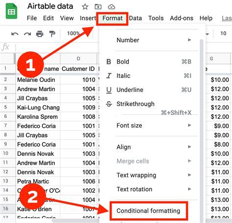
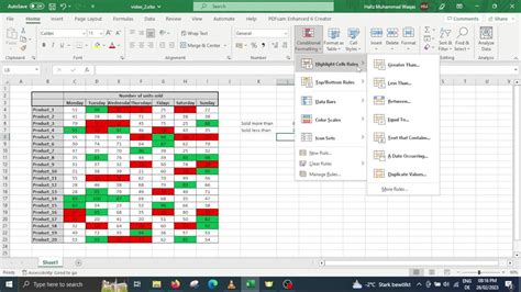
Using Conditional Formatting

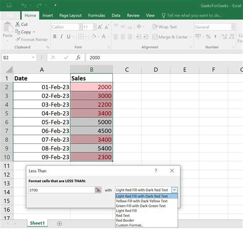
Conditional Formatting is another powerful tool in Excel for highlighting duplicates. It allows you to visually identify duplicate values without needing to write a formula.

Select the range of cells you want to check for duplicates.
Go to the Home tab on the Ribbon.
Click on Conditional Formatting.
Select Highlight Cells Rules, then Duplicate Values.
Choose a formatting style and click OK.

This method will highlight all duplicate values in the selected range, making it easy to spot them at a glance.

Advantages of Conditional Formatting

It's quick and easy to apply.
It provides a visual cue, making it easier to identify duplicates.
It does not alter the original data.

Using Array Formulas for Duplicate Check

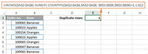
For more complex datasets or for users who prefer a formula-based approach, array formulas can offer a powerful solution. An array formula can return an array of values that indicate whether each value in a range is a duplicate.

=IF(FREQUENCY(range, range) > 1, "Duplicate", "Unique")

This formula uses the FREQUENCY function, which returns an array of frequencies for each value in the range. By checking if any frequency is greater than 1, you can identify duplicates.

Applying Array Formulas

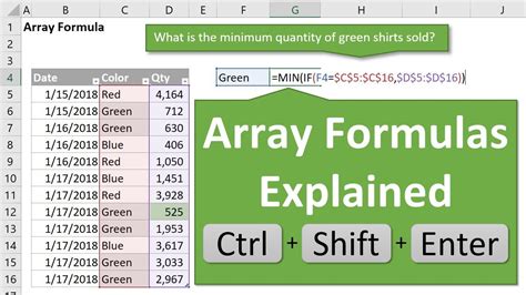
Select the cell where you want the result to appear.
Type the formula =IF(FREQUENCY(A:A, A:A) > 1, "Duplicate", "Unique"), assuming your data is in column A.
Press Ctrl+Shift+Enter instead of just Enter to apply the array formula.
The formula will return an array of results, indicating which values are duplicates.

Gallery of Excel Formulas for Duplicate Check

Excel Formulas Image Gallery

What is the simplest way to check for duplicates in Excel?

The simplest way is by using Conditional Formatting to highlight duplicate values.

How do I use the IF and COUNTIF functions to check for duplicates?

Use the formula =IF(COUNTIF(range, cell) > 1, "Duplicate", "Unique") to mark duplicates.

What is the purpose of using array formulas for duplicate checks?

Array formulas provide a powerful method for identifying duplicates, especially in complex datasets.

How do I apply Conditional Formatting to highlight duplicates?

Select the range, go to Home > Conditional Formatting > Highlight Cells Rules > Duplicate Values.

What are the benefits of checking for duplicates in Excel?

Checking for duplicates helps in data cleaning, ensures data integrity, and prevents incorrect analysis.

In conclusion, checking for duplicates in Excel is a crucial step in data analysis and management. With various formulas and tools available, from the IF and COUNTIF functions to Conditional Formatting and array formulas, users can efficiently identify and manage duplicates. Whether you're a beginner or an advanced Excel user, understanding how to check for duplicates can significantly enhance your data analysis capabilities. We invite you to share your experiences with duplicate checking in Excel, ask questions, or explore more topics related to data management and analysis. Your feedback and engagement are invaluable in creating a community that learns and grows together.