Excel Intersection Of Two Columns

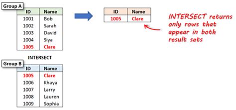
When working with data in Excel, identifying the intersection of two columns can be crucial for various analyses and tasks. This process involves finding the common elements or values that exist in both columns. Understanding how to achieve this is essential for data manipulation, filtering, and analysis. In this article, we will delve into the methods and techniques used to find the intersection of two columns in Excel, exploring both manual methods and formulas that can simplify this task.

Finding the intersection of two columns manually can be time-consuming and prone to errors, especially when dealing with large datasets. However, for small datasets or for understanding the basic concept, manual identification can be straightforward. You simply look through each column and identify any values that appear in both. This method, while simple, is not efficient for large datasets and does not leverage the powerful capabilities of Excel.

Using Formulas to Find Intersection

Excel offers several formulas that can be used to find the intersection of two columns more efficiently. One of the most common methods involves using the IF and MATCH functions together. The MATCH function looks for a value within a range and returns its relative position. By combining this with IF, you can check if a value from one column exists in another and return a corresponding value or a flag indicating a match.

For example, if you have two columns, A and B, and you want to find values in column A that also exist in column B, you could use a formula like this:

=IF(ISNUMBER(MATCH(A1, B:B, 0)), "Match", "No Match")

This formula checks if the value in cell A1 exists anywhere in column B. If it does, the formula returns "Match"; otherwise, it returns "No Match". You can apply this formula to each cell in column A to find intersections.

Using VLOOKUP for Intersection

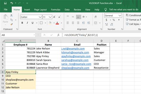
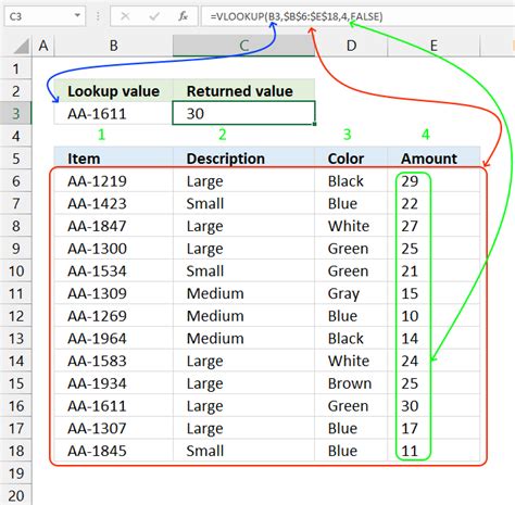
Another powerful function in Excel for finding intersections is VLOOKUP. The VLOOKUP function looks up a value in the first column of a table and returns a value in the same row from another column. While primarily used for looking up values, it can also be adapted to find intersections by checking if a lookup returns an error (indicating no match) or a value.

The syntax for VLOOKUP is:

VLOOKUP(lookup_value, table_array, col_index_num, [range_lookup])

To use VLOOKUP for finding intersections, you might use a formula like this:

=IF(ISERROR(VLOOKUP(A1, B:B, 1, FALSE)), "No Match", "Match")

This formula looks up the value in A1 within column B. If VLOOKUP finds a match, it returns the value itself (since col_index_num is 1), and the IF statement returns "Match". If no match is found, VLOOKUP returns an error, which the IF statement catches and returns "No Match".

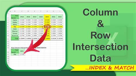
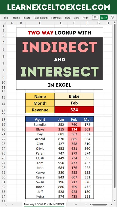
Using INDEX/MATCH for More Complex Intersections

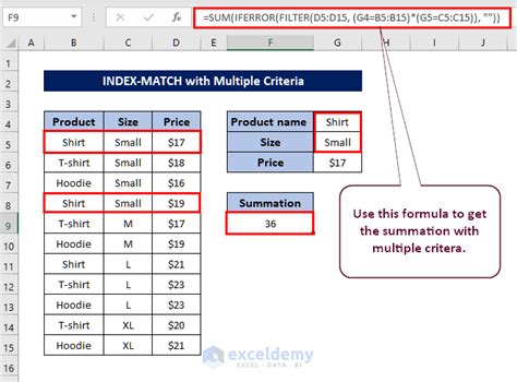
For more complex scenarios or when you need to return values based on intersections, the INDEX/MATCH function combination is incredibly powerful. This combination allows for lookups in any column or row and can handle multiple criteria.

The basic syntax for INDEX/MATCH is:

INDEX(range, MATCH(lookup_value, lookup_array, [match_type])

You can use this to find intersections by looking up values from one column in another and returning corresponding values from a third column, for example.

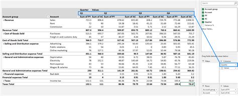
Using PivotTables for Intersection Analysis

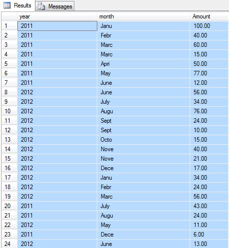
PivotTables are another Excel feature that can be used for intersection analysis, especially when dealing with large datasets. By creating a PivotTable and using the columns you're interested in as row and column labels, you can easily identify intersections and summarize data related to those intersections.

To create a PivotTable, go to the "Insert" tab in Excel, click on "PivotTable," and follow the prompts to set up your PivotTable. Then, drag the fields you want to analyze into the "Row Labels" and "Column Labels" areas of the PivotTable Fields pane.

Intersection of Multiple Columns

When dealing with more than two columns, finding the intersection involves identifying values that are common across all columns. This can be achieved by using nested IF functions or by leveraging more advanced Excel functions like FILTER (available in Excel 365 and later versions).

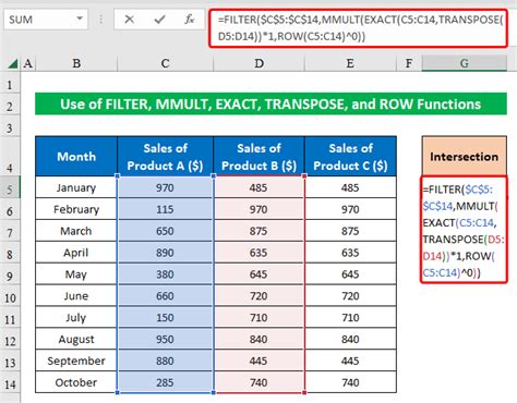
The FILTER function allows you to filter a range of data based on criteria. For finding intersections across multiple columns, you could use a formula like this:

=FILTER(A:A, (ISNUMBER(MATCH(A:A, B:B, 0))) * (ISNUMBER(MATCH(A:A, C:C, 0))))

This formula filters column A to show only values that exist in both columns B and C.

Gallery of Excel Intersection Examples

Excel Intersection Image Gallery

Frequently Asked Questions

What is the easiest way to find the intersection of two columns in Excel?

+

The easiest way often involves using formulas like IF and MATCH or VLOOKUP to identify common values.

Can I use PivotTables to find intersections?

+

Yes, PivotTables are very useful for analyzing intersections, especially in large datasets.

How do I find the intersection of multiple columns?

+

You can use nested IF functions or more advanced functions like FILTER to find intersections across multiple columns.

In conclusion, finding the intersection of two columns in Excel is a fundamental skill that can be achieved through various methods, from manual identification to using powerful formulas and features like PivotTables. By understanding and applying these techniques, you can efficiently analyze and manipulate your data, uncovering insights that might otherwise remain hidden. Whether you're working with small datasets or large, complex spreadsheets, mastering the art of finding intersections in Excel will significantly enhance your data analysis capabilities. We invite you to share your experiences, tips, or questions regarding Excel intersections in the comments below, and don't forget to share this article with anyone who might benefit from learning more about Excel's powerful data analysis features.