Google Sheets Index Match Formula

The Google Sheets Index Match formula is a powerful and flexible tool used for looking up and retrieving data from a table or range. Unlike the VLOOKUP function, which searches for a value in the first column of a table and returns a value in the same row from another column, the Index Match formula combination offers more versatility and is less prone to errors when the structure of the table changes. This is because it allows you to search for a value in any column and return a corresponding value from any other column.

The basic syntax of the Index Match formula involves two main functions: INDEX and MATCH. The MATCH function is used to find the position of a value within a range, while the INDEX function returns a value at a specific position within a range. When combined, these functions enable you to perform lookups that are not limited by the constraints of the VLOOKUP function.

To understand how to use the Index Match formula, let's break down its components and then explore how they are used together.

Introduction to the INDEX Function

The INDEX function returns a value at a specified position in a list or table. Its syntax is INDEX(range, row, column), where:

• range is the range of cells that you want to retrieve a value from.
• row is the row number in the range from which to return a value.
• column is the column number in the range from which to return a value.

If you only specify row, it returns the value in the specified row from the first column of the range. If you only specify column, it returns the value in the specified column from the first row of the range.

Introduction to the MATCH Function

The MATCH function searches for a value within a range and returns its relative position. The syntax is MATCH(lookup_value, lookup_array, [match_type]), where:

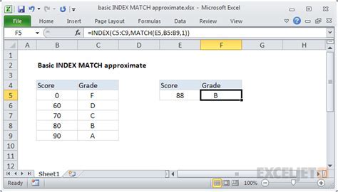
• lookup_value is the value you want to search for.
• lookup_array is the range of cells where you want to search for the value.
• [match_type] is optional and specifies whether you want an exact match or an approximate match. The default is an exact match (1), but you can also use 0 for an exact match, -1 for a value less than the lookup value, or 1 for a value greater than or equal to the lookup value.

Combining INDEX and MATCH

When you combine the INDEX and MATCH functions, you typically use the MATCH function to find the position of a value within a range (usually a column), and then use this position in the INDEX function to retrieve the corresponding value from another range (usually another column).

The general syntax for the Index Match formula is INDEX(return_range, MATCH(lookup_value, lookup_array, [match_type])), where:

• return_range is the range from which you want to return a value.
• lookup_value is the value you're looking for.
• lookup_array is the range where you're looking for the lookup_value.

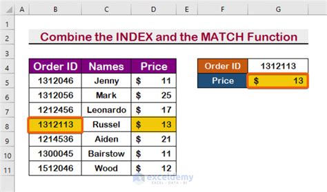
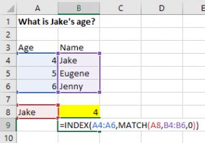
For example, if you have a table with names in column A and ages in column B, and you want to find the age of a person named "John", your formula might look like this:

=INDEX(B:B, MATCH("John", A:A, 0))

This formula searches for "John" in column A, finds its position, and then returns the value in the same position from column B.

Advantages of Using Index Match

1. Flexibility: Unlike VLOOKUP, which requires the lookup column to be the first column of the range, Index Match allows you to search in any column and return values from any other column.
2. Less Error-Prone: If the structure of your table changes (e.g., columns are inserted or deleted), the Index Match formula is less likely to break because it does not rely on column numbers.
3. Performance: In large datasets, Index Match can be faster than VLOOKUP because it uses relative positions rather than absolute column numbers.

Practical Examples

Example 1: Finding a Specific Value

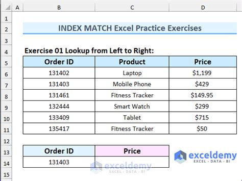
Suppose you have a list of products in column A and their prices in column B. You want to find the price of a product named "Product X".

=INDEX(B:B, MATCH("Product X", A:A, 0))

Example 2: Using Index Match with Multiple Criteria

If you need to find a value based on multiple criteria, you can use the INDEX and MATCH functions in combination with the FILTER function (available in Google Sheets) or by using an array formula with the INDEX and MATCH functions.

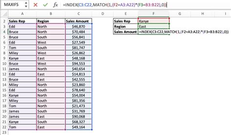
For instance, to find the price of "Product Y" from a specific supplier "Supplier Z", assuming products are in column A, suppliers in column B, and prices in column C, you could use an array formula like this:

=INDEX(C:C, MATCH(1, (A:A="Product Y") * (B:B="Supplier Z"), 0))

Note: This formula needs to be entered by pressing Ctrl+Shift+Enter (or Cmd+Shift+Enter on a Mac) instead of just Enter, to make it an array formula.

Tips and Variations

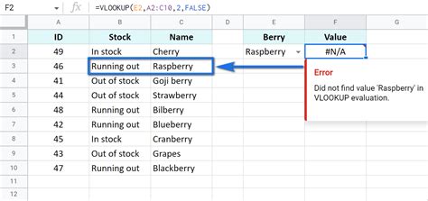
• Using Wildcards: You can use wildcards (* or ?) in the lookup_value of the MATCH function to search for patterns. For example, MATCH("Jo*", A:A, 0) would find any value starting with "Jo".
• Handling Errors: If the value is not found, the MATCH function returns a #N/A error. You can handle this by wrapping your formula in an IFERROR function, like =IFERROR(INDEX(B:B, MATCH("John", A:A, 0)), "Not Found").
• Multi-Dimensional Lookup: For more complex lookups involving multiple tables or conditions, consider using the FILTER function or QUERY function in Google Sheets, which can offer more straightforward solutions than nested INDEX and MATCH functions.

Conclusion and Next Steps

The Google Sheets Index Match formula is a powerful tool for data analysis and retrieval. Its flexibility and ability to handle lookups in any column make it a preferred choice over VLOOKUP for many users. By mastering the INDEX and MATCH functions, you can perform a wide range of data manipulation tasks in Google Sheets, from simple lookups to complex data analysis. Whether you're working with personal finance, managing inventory, or analyzing customer data, the Index Match formula can help you extract the insights you need from your data.

Advanced Index Match Techniques

For those looking to dive deeper into the capabilities of the Index Match formula, exploring advanced techniques such as using multiple criteria, handling errors, and combining with other Google Sheets functions can significantly enhance your data analysis capabilities.

Using Index Match with Other Google Sheets Functions

The versatility of the Index Match formula is further expanded when combined with other powerful functions in Google Sheets, such as FILTER, QUERY, and VLOOKUP. Understanding how to integrate these functions can help you tackle complex data challenges with ease.

Best Practices for Using Index Match

To get the most out of the Index Match formula and ensure your spreadsheets remain efficient and easy to maintain, following best practices such as keeping your data organized, using absolute references when necessary, and testing your formulas thoroughly is essential.

Troubleshooting Common Index Match Errors

Despite its power, the Index Match formula can sometimes return errors, especially if the data is not properly formatted or if the formula is not correctly constructed. Knowing how to troubleshoot these errors can save you time and frustration.

Conclusion on Mastering Index Match

Mastering the Index Match formula is a significant step towards becoming proficient in Google Sheets. By understanding its capabilities, limitations, and best practices, you can unlock a wide range of data analysis possibilities and make your work with spreadsheets more efficient and effective.

Index Match Formula Gallery

What is the main advantage of using the Index Match formula over VLOOKUP?

+

The main advantage is its flexibility and less error-prone nature, as it allows searching in any column and returning values from any other column without relying on column numbers.

How do I handle errors when using the Index Match formula?

+

You can handle errors by wrapping your formula in an IFERROR function, specifying a value to return if the lookup value is not found, such as "Not Found" or a blank string.

Can I use the Index Match formula for multi-dimensional lookups?

+

Yes, you can use the Index Match formula for multi-dimensional lookups by combining it with other functions like FILTER or by using array formulas that can handle multiple criteria.

We hope this comprehensive guide to the Google Sheets Index Match formula has been informative and helpful. Whether you're a beginner looking to understand the basics or an advanced user seeking to refine your skills, mastering the Index Match formula can significantly enhance your productivity and data analysis capabilities in Google Sheets. Feel free to share your experiences, ask questions, or provide tips on using the Index Match formula in the comments below.