Intro
Sorting data in Excel pivot tables is a crucial skill for anyone looking to analyze and summarize large datasets efficiently. Pivot tables offer a powerful way to rotate, aggregate, and summarize data, making it easier to understand and draw insights from it. One of the fundamental operations you might want to perform on your pivot table data is sorting it from highest to lowest. This can help in identifying top performers, highest values, or most significant changes within your dataset. In this article, we will delve into the steps and methods to sort your pivot table data from highest to lowest, exploring various scenarios and providing practical examples.
When working with pivot tables, the ability to sort and filter data becomes indispensable. It allows you to focus on the most critical aspects of your data, whether it's sales figures, customer demographics, or product performance metrics. Sorting from highest to lowest can be particularly useful in highlighting trends, outliers, and areas that require immediate attention. Before we dive into the sorting process, let's briefly cover the basics of creating a pivot table and why sorting is an essential feature.
Understanding Pivot Tables
Pivot tables are a tool in Excel that allows you to summarize and analyze large datasets. They enable you to rotate and aggregate data, creating custom views that can help in understanding complex data relationships. Pivot tables consist of fields that can be dragged and dropped into areas such as rows, columns, and values. The values area is where you typically place fields you want to summarize or aggregate, such as sum, average, or count.
Creating a Pivot Table
To create a pivot table, you start by selecting a cell in your dataset, then navigate to the "Insert" tab in the Excel ribbon, and click on "PivotTable." Excel will prompt you to choose a cell to place your pivot table and select the data range you wish to analyze. Once your pivot table is set up, you can begin customizing it by adding fields to the rows, columns, and values areas.
Sorting Pivot Table Data
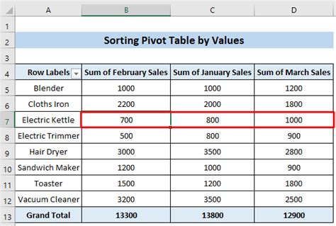
Sorting data in a pivot table can be done in several ways, depending on whether you want to sort based on the row labels, column labels, or the values themselves. Here, we focus on sorting the values from highest to lowest.
Sorting Values from Highest to Lowest
- Select the Pivot Table: Click anywhere inside your pivot table to activate it.
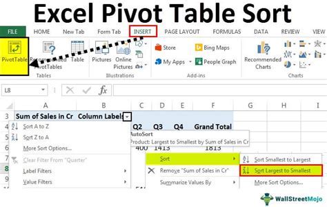
- Right-Click on the Value: Right-click on the value you want to sort within the pivot table. This could be a sum, count, or any other aggregated value.
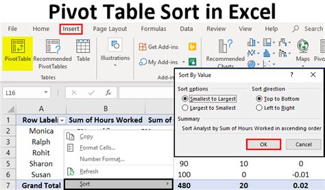
- Select "Sort" and Then "Sort Descending": From the context menu, navigate to "Sort" and then select "Sort Descending." This will sort your data in descending order, placing the highest values first.
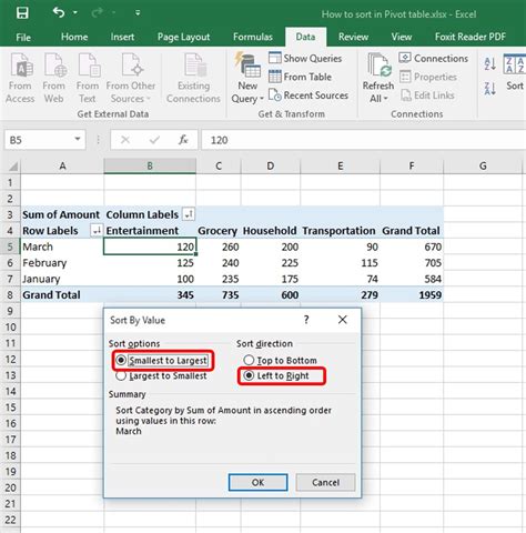
Alternatively, you can use the "Sort & Filter" option in the "Data" tab of the Excel ribbon. After selecting your pivot table, go to the "Data" tab, click on "Sort & Filter," and then choose "Custom Sort." In the sort dialog box, select the column or field you want to sort, choose "Descending" under "Order," and click "OK."
Sorting Row Labels
If you want to sort based on the row labels, you can do so directly from the pivot table fields list.
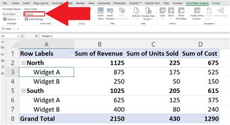
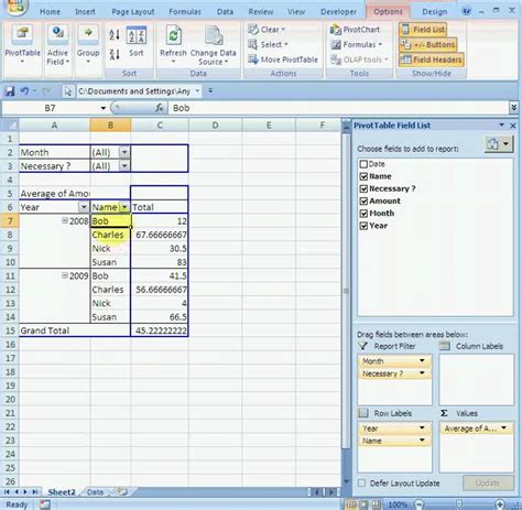
- Open the PivotTable Fields List: If the PivotTable Fields list is not visible, go to the "Analyze" tab in the Excel ribbon and click on "Field List."
- Drag a Field to the "Row Labels" Area: Ensure the field you want to sort by is in the "Row Labels" area.
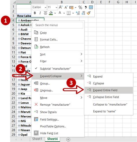
- Right-Click on the Row Label: Right-click on the row label you wish to sort.
- Select "Sort" and Then "Sort A to Z" or "Sort Z to A": Depending on whether you want to sort alphabetically from A to Z (ascending) or Z to A (descending), make your selection.
Advanced Sorting Techniques
In some cases, you might need to perform more complex sorting operations, such as sorting by multiple fields or using custom sorting lists.
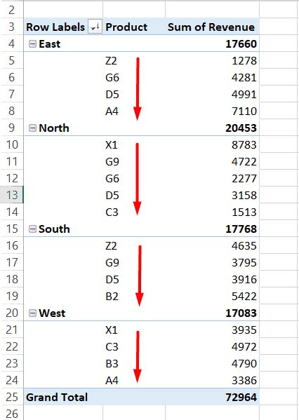
Sorting by Multiple Fields
- Select the Field: Right-click on the field you wish to sort.
- Select "Sort" and Then "More Sort Options": This opens the "Sort" dialog box.
- Add Levels: Click on "Add Level" to add another field to sort by.
- Then By: Select the next field you want to sort by from the "Then by" dropdown.
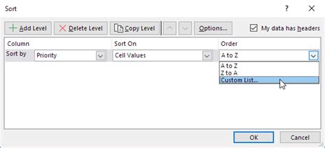
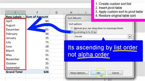
Using Custom Sorting Lists
Excel allows you to create custom lists for sorting, which can be particularly useful if you have specific categories or priorities you want to apply to your data.
- Go to File > Options: Navigate to the Excel options.
- Select "Advanced": Scroll down to the "General" section.
- Click on "Edit Custom Lists": This opens the "Custom Lists" dialog box.
- New List: Enter your custom list and click "Add."
Tips for Effective Pivot Table Sorting
- Keep Your Data Organized: Ensure your source data is well-structured and clean to get the most out of your pivot table sorting.
- Use Pivot Table Filters: In addition to sorting, use filters to narrow down your data and focus on specific subsets.
- Refresh Your Pivot Table: After making changes to your source data, don't forget to refresh your pivot table to reflect the updates.

Gallery of Pivot Table Sorting Examples
Pivot Table Sorting Gallery


FAQs
How do I sort a pivot table in Excel?
+To sort a pivot table, right-click on the field you wish to sort, select "Sort," and then choose either "Sort Ascending" or "Sort Descending" depending on your preference.
Can I sort a pivot table by multiple fields?
+Yes, you can sort a pivot table by multiple fields. Right-click on the field, select "Sort" and then "More Sort Options," and use the "Add Level" feature to add additional fields to sort by.
How do I create a custom sorting list in Excel?
+To create a custom sorting list, go to File > Options, select "Advanced," and click on "Edit Custom Lists." Then, enter your list and click "Add" to create a new custom list for sorting.
In conclusion, sorting pivot table data from highest to lowest is a straightforward yet powerful technique for data analysis in Excel. By mastering the various methods of sorting, including sorting values, row labels, and using custom lists, you can unlock deeper insights into your data and make more informed decisions. Remember to keep your data organized, utilize pivot table filters, and refresh your pivot tables regularly to ensure your analyses are always up-to-date. With practice and experience, you'll become proficient in leveraging pivot tables to uncover trends, patterns, and opportunities hidden within your data.