Intro
Learn how to use Excel return values matching criteria with functions like VLOOKUP, INDEX/MATCH, and IF statements to retrieve specific data, enabling efficient data analysis and lookup operations.
When working with Excel, one of the most powerful features is the ability to return values based on specific criteria. This can be achieved through various functions, including VLOOKUP, INDEX/MATCH, and FILTER. Understanding how to use these functions can significantly enhance your data analysis and manipulation capabilities in Excel.
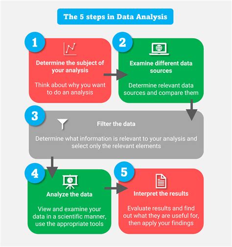
The importance of returning values based on criteria lies in its ability to extract specific information from large datasets. This can be crucial for data analysis, reporting, and decision-making. For instance, in a sales database, you might want to find the sales amount for a specific product in a particular region. By using functions that return values based on criteria, you can easily retrieve this information without having to manually sift through the data.
Excel's functionality for returning values based on criteria is vast and can be applied in numerous scenarios. From simple tasks like finding a specific value in a list to complex data analysis involving multiple criteria, Excel's array of functions makes it a versatile tool for data management. As we delve into the specifics of these functions, it becomes clear that mastering them can greatly improve productivity and accuracy in data handling.
Understanding VLOOKUP
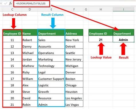
VLOOKUP is one of the most commonly used functions in Excel for returning values based on criteria. It stands for "vertical lookup" and is used to find a value in a table based on a lookup value. The syntax for VLOOKUP is VLOOKUP(lookup_value, table_array, col_index_num, [range_lookup]). The lookup_value is the value you want to look up, table_array is the range of cells that contains the data, col_index_num is the column number that contains the return value, and [range_lookup] is optional and specifies whether you want an exact match or an approximate match.
How VLOOKUP Works
VLOOKUP works by searching for the `lookup_value` in the first column of the `table_array`. Once it finds a match, it returns the value in the same row from the column specified by `col_index_num`. If `[range_lookup]` is set to FALSE, VLOOKUP will look for an exact match. If it's set to TRUE or omitted, VLOOKUP will look for an approximate match, which means it will find the largest value that is less than or equal to the `lookup_value`.Using INDEX/MATCH for Returning Values
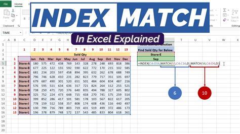
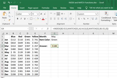
The INDEX/MATCH function combination is another powerful tool for returning values based on criteria. It is often preferred over VLOOKUP because it is more flexible and can handle more complex lookups. The syntax for INDEX/MATCH is INDEX(range, MATCH(lookup_value, lookup_array, [match_type]), where range is the range of cells from which to return a value, lookup_value is the value you want to look up, lookup_array is the range of cells that contains the data to search, and [match_type] specifies whether you want an exact match or an approximate match.
Advantages of INDEX/MATCH
One of the main advantages of using INDEX/MATCH over VLOOKUP is that it allows for lookups in any column, not just the first column. Additionally, INDEX/MATCH is less prone to errors when columns are inserted or deleted, as it references columns by their position relative to the lookup array, rather than by a fixed column number.Introducing the FILTER Function

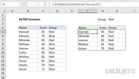
The FILTER function is a newer addition to Excel's array of functions for returning values based on criteria. It allows you to filter a range of data based on criteria and return the filtered values. The syntax for FILTER is FILTER(array, include, [if_empty]), where array is the range of cells to filter, include is a logical expression that determines which cells to include, and [if_empty] is an optional argument that specifies what to return if the filter returns no results.
Using FILTER for Dynamic Data Analysis
The FILTER function is particularly useful for dynamic data analysis, where the criteria for filtering data may change frequently. It can be used in conjunction with other functions, such as the `AND` and `OR` functions, to create complex filter criteria. Additionally, FILTER can be used with arrays, making it a powerful tool for handling large datasets.Practical Applications and Examples
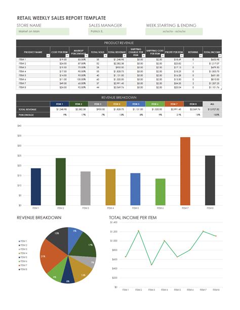
Understanding how to return values based on criteria in Excel opens up a wide range of practical applications. For instance, in a sales report, you might use VLOOKUP to find the sales amount for a specific product, or use INDEX/MATCH to find the sales amount for a product in a specific region. The FILTER function can be used to dynamically filter a list of sales data based on criteria such as product category, region, or sales amount.
Step-by-Step Examples
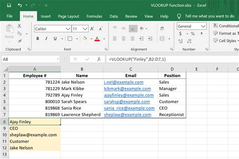
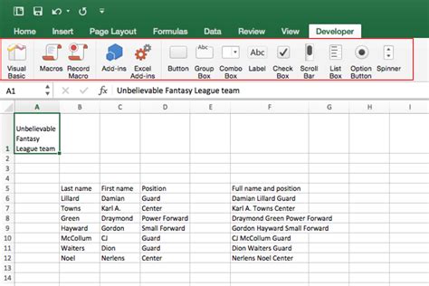
Here are some step-by-step examples to illustrate how to use these functions: - **VLOOKUP Example**: Suppose you have a table with employee names in the first column and their corresponding salaries in the second column. You can use VLOOKUP to find an employee's salary by their name. - **INDEX/MATCH Example**: If you have a table with product names in one column and prices in another, you can use INDEX/MATCH to find the price of a specific product. - **FILTER Example**: If you have a list of sales data and you want to see only the sales for a specific region, you can use the FILTER function to dynamically filter the data.Gallery of Excel Functions
Excel Functions Gallery


Frequently Asked Questions
What is the main difference between VLOOKUP and INDEX/MATCH?
+VLOOKUP searches for a value in the first column of a table and returns a value in the same row from another column, while INDEX/MATCH allows for lookups in any column and is more flexible.
How do I use the FILTER function in Excel?
+The FILTER function is used to filter a range of data based on criteria. The syntax is FILTER(array, include, [if_empty]), where array is the range to filter, include is the criteria, and [if_empty] is what to return if no results are found.
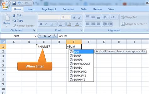
What are some common errors to avoid when using VLOOKUP?
+Common errors include referencing the wrong column, not using absolute references for the table array, and not handling errors for when the lookup value is not found.
In conclusion, mastering the art of returning values based on criteria in Excel can significantly enhance your data analysis capabilities. Whether you're using VLOOKUP, INDEX/MATCH, or the FILTER function, understanding how to apply these functions can help you extract specific information from large datasets with ease. As you continue to explore the depths of Excel's functionality, remember that practice makes perfect, and experimenting with different scenarios will help solidify your understanding of these powerful tools. Feel free to share your experiences or ask questions about using these functions in the comments below, and don't forget to share this article with anyone who might benefit from learning more about Excel's capabilities for returning values based on criteria.