Intro
Get column letters in Google Sheets with ease. Learn how to convert column numbers to letters and vice versa using formulas and scripts, making data analysis and spreadsheet management more efficient with column letter referencing.
The versatility of Google Sheets offers numerous functions to manipulate and analyze data efficiently. One common requirement when working with spreadsheets is the ability to convert column numbers to their corresponding letters, which can be particularly useful in scripting, referencing, or even in formulas. Google Sheets provides a straightforward method to achieve this conversion using its built-in functions. Let's delve into how you can get the column letter from a column number in Google Sheets.
Introduction to Column Letters in Google Sheets
In Google Sheets, columns are identified by letters (A, B, C, etc.), while rows are identified by numbers. This lettering system continues up to column Z, after which it moves to AA, AB, AC, and so on, similar to how the alphabet works. When you're working with scripts or formulas that require you to dynamically reference columns, knowing how to convert a column number to its corresponding letter is invaluable.
Using the COLUMN Function
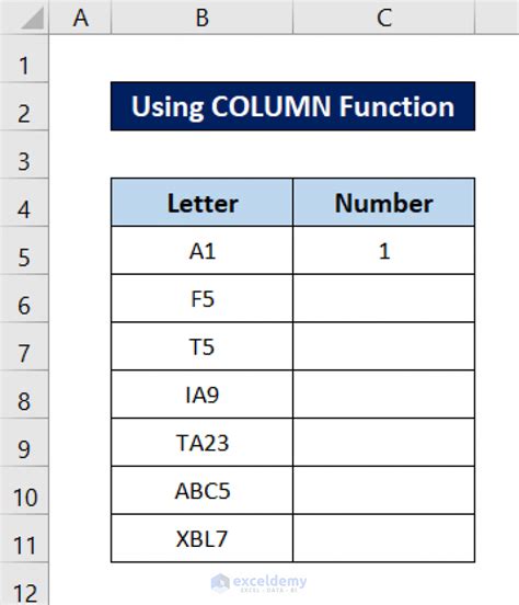
Before diving into the conversion, it's useful to know how to get the column number of a cell. The COLUMN function in Google Sheets returns the column number of a reference. For example, if you input =COLUMN(A1), the function will return 1, because A is the first column.
Converting Column Number to Letter
To convert a column number to its corresponding letter, you can use a combination of the CHAR and INT functions along with some arithmetic. The formula to achieve this conversion is as follows:
=CHAR(64+COLUMN(A1))
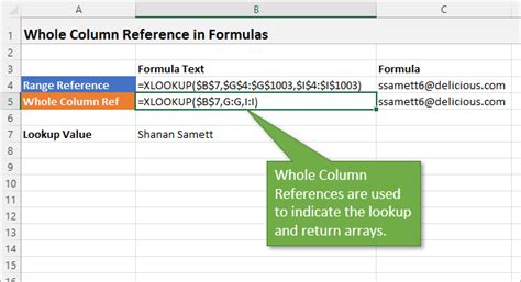
However, this formula only works for columns up to Z (column 26). For columns beyond Z, you need a more complex formula that can handle the alphabetical progression (AA, AB, etc.). Here's a formula that works for any column:
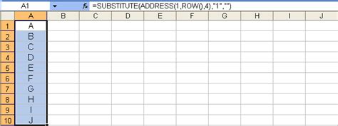
=SUBSTITUTE(ADDRESS(1,COLUMN(A1),4),"1","")
This formula uses the ADDRESS function to generate a cell reference in the format of $A$1, and then it uses the SUBSTITUTE function to remove the row number (1) and the dollar signs, leaving just the column letter.
Practical Applications
Understanding how to convert between column numbers and letters is not just a theoretical exercise; it has several practical applications:
- Dynamic References: In scripts or complex formulas, you might need to reference columns dynamically based on user input or calculations. Converting column numbers to letters allows you to create these dynamic references.
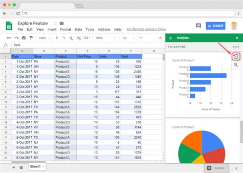
- Data Analysis: When analyzing data, being able to quickly identify and reference specific columns can significantly streamline your workflow.
- Automation: In Google Apps Script, converting column numbers to letters can be crucial for automating tasks that involve iterating over columns or referencing specific columns based on conditions.
Steps to Implement the Conversion
- Identify Your Column Number: First, determine the column number you want to convert. If you're starting from a cell reference, you can use the COLUMN function as mentioned earlier.
- Apply the Conversion Formula: Use the appropriate formula based on whether you expect to work with columns only up to Z or beyond. For most cases, the second formula that uses the ADDRESS and SUBSTITUTE functions will be more versatile.
- Adjust as Necessary: Depending on your specific use case, you might need to adjust the formula. For example, if you're working within a script, you'll need to adapt the formula to work with the script's syntax and data types.
Example Use Cases
- Simple Conversion: If you want to convert column 5 to its letter equivalent, you would use the formula
=SUBSTITUTE(ADDRESS(1,5,4),"1",""), which returnsE. - Dynamic Column Reference: Suppose you have a value in cell A1 that represents a column number, and you want to reference the header in that column. You could use
=SUBSTITUTE(ADDRESS(1,A1,4),"1","")to get the column letter and then concatenate it with "1" (for the first row) to create a cell reference like$E$1.
Gallery of Column Conversion


Gallery of Google Sheets
Google Sheets Gallery


FAQs
How do I convert a column number to a letter in Google Sheets?
+You can use the formula =SUBSTITUTE(ADDRESS(1,COLUMN(A1),4),"1","") to convert a column number to its corresponding letter.
What is the COLUMN function used for in Google Sheets?
+The COLUMN function returns the column number of a reference. For example, =COLUMN(A1) returns 1, because A is the first column.
How do I dynamically reference a column in Google Sheets based on a value?
+You can use the INDIRECT function along with the column letter conversion formula to dynamically reference a column. For example, if A1 contains the column number, you can use =INDIRECT(SUBSTITUTE(ADDRESS(1,A1,4),"1","")&"1") to reference the cell in the specified column and row 1.
In conclusion, converting column numbers to letters in Google Sheets is a valuable skill that can enhance your spreadsheet management and analysis capabilities. By understanding and applying the formulas and techniques outlined in this article, you can more efficiently work with your data and automate tasks to improve productivity. Whether you're a beginner or an advanced user, mastering these skills can significantly impact how you interact with Google Sheets and solve problems within your spreadsheets.