Highlight Row If Cell Contains Text Google Sheets

Highlighting rows in Google Sheets based on specific conditions, such as if a cell contains certain text, can be incredibly useful for data analysis and visualization. This feature helps in quickly identifying key information, patterns, or anomalies within your dataset. Google Sheets provides several ways to achieve this, including using conditional formatting, formulas, and scripts. Here, we'll explore how to highlight rows if a cell contains specific text using these methods.

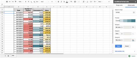
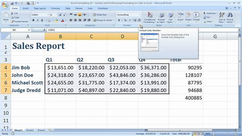
Using Conditional Formatting

Conditional formatting is the most straightforward way to highlight rows based on the content of cells. Here's how you can do it:

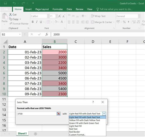
Select the Range: Click and drag your mouse to select the entire range of cells you want to apply the formatting to, including headers if you want them to be part of the selection.
Open Conditional Format: Go to the "Format" tab in the menu, hover over "Conditional formatting," and click on it.
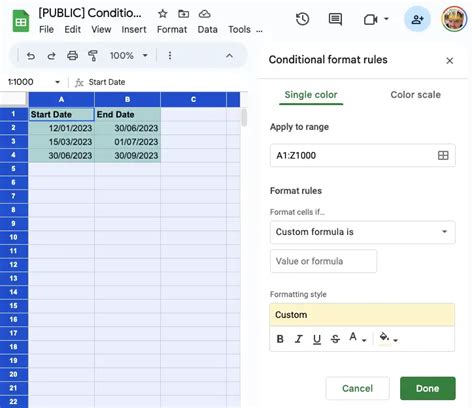
Apply Custom Formula: In the format cells if dropdown, select "Custom formula is".
Enter Formula: In the formula bar, you can enter a formula like =REGEXMATCH(A1, "text") if you want to highlight rows where the cell in column A contains the word "text". Replace "A1" with the first cell of your range and "text" with the word you're looking for.
Apply to Range: Make sure the range is correctly selected in the "Apply to range" field. If you've selected a range before opening the conditional formatting tool, this should be filled in automatically.
Format: Choose how you want the highlighted rows to look by clicking on the "Format" button and selecting your preferences (background color, font color, etc.).
Done: Click "Done" to apply the formatting.

This method will automatically highlight any row where the specified condition (in this case, containing specific text) is met in the selected column.

Using Google Apps Script

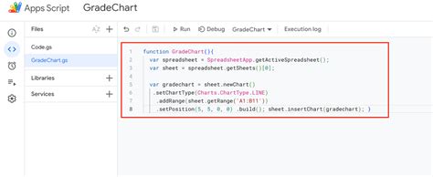
For more complex operations or if you prefer a programmatic approach, you can use Google Apps Script. This method allows for more flexibility and can be triggered automatically based on edits or at specific times.

Open Script Editor: Go to "Tools" > "Script editor" in your Google Sheet.
Write Script: You can write a script that iterates through your data and applies formatting based on conditions. For example:

function highlightRows() {
  var sheet = SpreadsheetApp.getActiveSpreadsheet().getActiveSheet();
  var range = sheet.getDataRange();
  var values = range.getValues();
  
  for (var i = 0; i < values.length; i++) {
    if (values[i][0].toString().indexOf("text")!== -1) { // Checks if the first column contains "text"
      sheet.getRange(i + 1, 1, 1, range.getLastColumn()).setBackground("yellow"); // Highlights the entire row
    }
  }
}

Replace "text" with the text you're searching for, and adjust the column index in values[i][0] if you're checking a different column.

Run Script: You can run this script manually from the script editor or set up a trigger to run it automatically.

Practical Examples

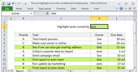
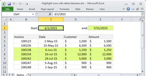
Highlighting Rows with Specific Keywords: Suppose you have a list of products and their descriptions in column A, and you want to highlight rows where the description contains the word "sale". You can use the formula =REGEXMATCH(A1, "sale") in conditional formatting.
Highlighting Rows Based on Multiple Conditions: If you need to highlight rows based on multiple conditions (e.g., containing "sale" and "new"), you can modify the formula to =REGEXMATCH(A1, "sale") * REGEXMATCH(A1, "new").

Statistical Data and Readability

When highlighting rows based on specific text, it's essential to consider the statistical implications of your data and how the highlighting affects readability. For instance, if a large number of rows are highlighted, it might not be as effective for drawing attention to specific data points. In such cases, you might want to refine your conditions or use additional formatting options to differentiate between various types of highlighted data.

Gallery of Highlighting Examples

Alternatives to Excel for highlighting rows

Gallery Section

Highlighting Rows Image Gallery

FAQs

How do I highlight rows in Google Sheets based on specific text?

You can use conditional formatting with a custom formula like `=REGEXMATCH(A1, "text")` to highlight rows where the cell in column A contains the word "text".

Can I use Google Apps Script to highlight rows automatically?

Yes, you can write a script that checks for specific conditions in your data and applies highlighting accordingly. This can be set to run automatically based on edits or at specific times.

How do I refine my conditions for highlighting rows to make it more specific?

You can modify your formulas or scripts to include more specific conditions, such as looking for multiple keywords or excluding certain phrases. This can help in making your highlighting more targeted and useful.

Final Thoughts

Highlighting rows in Google Sheets based on specific text is a powerful tool for data analysis and visualization. Whether you're using conditional formatting, formulas, or scripts, the key to effective highlighting is to clearly define your conditions and ensure that the formatting enhances the readability and understanding of your data. By mastering these techniques, you can unlock more insights from your data and present your findings in a more compelling and professional manner. Feel free to share your experiences or ask further questions in the comments below, and don't forget to share this article with others who might find it helpful.