Intro
The ability to sum filtered cells in Excel is a crucial skill for anyone working with large datasets. Filtering data allows you to narrow down your dataset to only the most relevant information, and being able to perform calculations on this filtered data can help you gain valuable insights. In this article, we will explore the various methods for summing filtered cells in Excel, including using formulas, pivot tables, and other tools.
When working with filtered data, it's essential to understand how Excel handles calculations. By default, Excel only includes visible cells in calculations, which means that if you have filtered out certain rows or columns, they will not be included in your calculations. This can be both beneficial and limiting, depending on your specific needs.
To get the most out of your data, you need to know how to harness the power of Excel's filtering and calculation tools. Whether you're a beginner or an advanced user, this article will provide you with the knowledge and skills you need to sum filtered cells in Excel with ease.
Using Formulas to Sum Filtered Cells
One of the most common methods for summing filtered cells is by using formulas. Excel provides several formulas that can help you achieve this, including the SUMIF and SUMIFS functions. The SUMIF function allows you to sum a range of cells based on a single criteria, while the SUMIFS function enables you to sum a range of cells based on multiple criteria.
To use the SUMIF function, you need to specify the range of cells that you want to sum, the criteria range, and the criteria itself. For example, if you want to sum all the values in column A that are greater than 10, you can use the following formula: =SUMIF(A1:A10, ">10").
On the other hand, the SUMIFS function allows you to specify multiple criteria ranges and criteria. For example, if you want to sum all the values in column A that are greater than 10 and less than 20, you can use the following formula: =SUMIFS(A1:A10, A1:A10, ">10", A1:A10, "<20").
Using Pivot Tables to Sum Filtered Cells
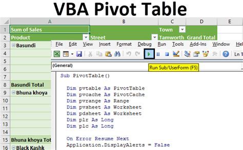
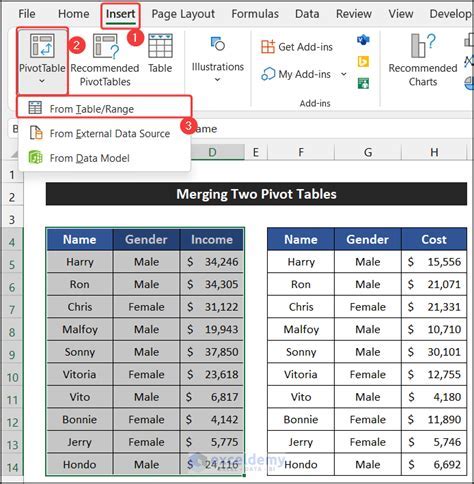
Pivot tables are another powerful tool in Excel that can help you sum filtered cells. A pivot table is a summary of a large dataset that can be rotated to show different fields and summaries. To create a pivot table, you need to select the range of cells that you want to summarize, go to the "Insert" tab, and click on "PivotTable".
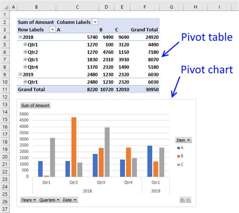
Once you have created a pivot table, you can use the "Row Labels" and "Column Labels" areas to filter your data. You can also use the "Values" area to specify the field that you want to sum. For example, if you want to sum all the values in column A, you can drag the "A" field to the "Values" area.
Steps to Create a Pivot Table
To create a pivot table, follow these steps:
- Select the range of cells that you want to summarize.
- Go to the "Insert" tab and click on "PivotTable".
- Choose a cell where you want to place the pivot table.
- Click "OK" to create the pivot table.
- Drag the fields that you want to use to the "Row Labels", "Column Labels", and "Values" areas.
Using the SUBTOTAL Function to Sum Filtered Cells
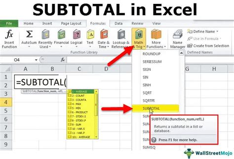
The SUBTOTAL function is another formula that can help you sum filtered cells. This function allows you to sum a range of cells and ignore any hidden rows or columns. To use the SUBTOTAL function, you need to specify the range of cells that you want to sum and the function number that corresponds to the SUM function.
For example, if you want to sum all the values in column A, you can use the following formula: =SUBTOTAL(109, A1:A10). The "109" in this formula corresponds to the SUM function, and the "A1:A10" specifies the range of cells that you want to sum.
Function Numbers for the SUBTOTAL Function
Here are some common function numbers that you can use with the SUBTOTAL function:
- 1: AVERAGE
- 2: COUNT
- 3: COUNTA
- 4: MAX
- 5: MIN
- 6: PRODUCT
- 7: STDEV
- 8: STDEVP
- 9: SUM
- 10: VAR
- 11: VARP
Using the AGGREGATE Function to Sum Filtered Cells
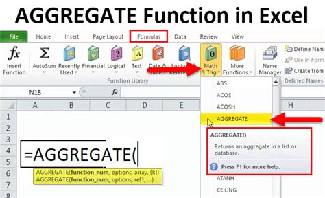
The AGGREGATE function is a more advanced formula that can help you sum filtered cells. This function allows you to sum a range of cells and ignore any errors or hidden rows or columns. To use the AGGREGATE function, you need to specify the range of cells that you want to sum, the function number that corresponds to the SUM function, and the option that specifies how to handle errors or hidden rows or columns.
For example, if you want to sum all the values in column A and ignore any errors, you can use the following formula: =AGGREGATE(1, 2, A1:A10). The "1" in this formula corresponds to the SUM function, the "2" specifies that you want to ignore any errors, and the "A1:A10" specifies the range of cells that you want to sum.
Options for the AGGREGATE Function
Here are some common options that you can use with the AGGREGATE function:
- 0: Ignore nothing
- 1: Ignore hidden rows and columns
- 2: Ignore errors
- 3: Ignore both hidden rows and columns and errors
- 4: Ignore nothing, including hidden rows and columns
- 5: Ignore hidden rows and columns, including structured references
- 6: Ignore errors, including #N/A
- 7: Ignore both hidden rows and columns and errors, including #N/A
Excel Formulas Image Gallery


What is the difference between the SUMIF and SUMIFS functions in Excel?
+The SUMIF function allows you to sum a range of cells based on a single criteria, while the SUMIFS function enables you to sum a range of cells based on multiple criteria.
How do I create a pivot table in Excel?
+To create a pivot table, select the range of cells that you want to summarize, go to the "Insert" tab, and click on "PivotTable". Choose a cell where you want to place the pivot table and click "OK" to create it.
What is the purpose of the SUBTOTAL function in Excel?
+The SUBTOTAL function allows you to sum a range of cells and ignore any hidden rows or columns.
In conclusion, summing filtered cells in Excel can be achieved through various methods, including using formulas, pivot tables, and other tools. By mastering these techniques, you can unlock the full potential of your data and gain valuable insights that can inform your business decisions. Whether you're a beginner or an advanced user, this article has provided you with the knowledge and skills you need to sum filtered cells in Excel with ease. So why not give it a try and see the difference it can make for yourself? Share your experiences and tips in the comments below, and don't forget to share this article with your friends and colleagues who may benefit from it.